File:Steps towards general relativity lecture.pdf

Original file (1,216 × 1,625 pixels, file size: 1.99 MB, MIME type: application/pdf, 295 pages)
| This is a file from the Wikimedia Commons. The description on its description page there is shown below.
Commons is a freely licensed media file repository. You can help. |
| Description |
English: This file is the (steps towards) general relativity lecture of the Wikiversity:Special relativity and steps towards general relativity course. It is in pdf format for convenient viewing as a fullscreen, structured presentation in a classroom. It uses encapsulated postscript versions of many Wikimedia Commons diagrams, using their .fig or octave source code when available. Most diagrams are labelled with mathematical expressions, using LaTeX "specials". The pdf contains many links to Wikipedia resources for more in-depth learning. Mediawiki-text and svg might become directly usable in the long term, but do not yet seem ready to replace LaTeX. |
| Date | |
| Source | Own work plus Wikimedia Commons files available under CC-BY-SA or public domain or GFDL licences, plus File:Commons-logo-en.svg (which is trademarked) to indicate to readers that images are from WM Commons. This logo usage seems likely to be acceptable, but the pdf file could easily be recreated without the logo if needed. A script for creating the pdf file and checking the licences of included (format converted) files will be added a few minutes after the main upload. The GFDL files seem to satisfy the CC-BY-SA compatibility operation. |
| Author | User:Boud |
| Permission (Reusing this file) |
This file is licensed under the Creative Commons Attribution-Share Alike 3.0 Unported license.
However, modifications need to either remove File:Commons-logo-en.svg from the file or be careful to continue following Wikimedia Foundation trademark policy regarding the logo. |
| Other versions |
related:  |
script and LaTeX source
The pdf file can be produced with the script and LaTeX source below.
shell script
This script is intended for users with the necessary GNU/Linux command line experience to understand what the script does and to modify it for personal usage.
- Do not use it without understanding what it does.
- Check this wiki page history to see who edited it, when they edited it, and what changes they made.
- See the disclaimer linked to at the bottom of this page.
Having got through the warnings, you are most welcome to improve the script.
#!/bin/bash
## (c) CC-BY-SA-3.0 and/or GPLv3 at your choosing
## See the Wikimedia Foundation Commons website for authorship.
## http://commons.wikimedia.org/wiki/File:Special_relativity_lecture.pdf
## http://commons.wikimedia.org/wiki/File:Steps_towards_general_relativity_lecture.pdf
## Changelog
##
## 2012-05-15 download_non_svg, etc: generalise sed expression in each
## URL=... because some absolute URLs are written without "http:"
## in (at least) the Commons html files;
## download_pdf: make ampersand, greater than, less than to appear
## correctly in the browser-rendered version of this script instead
## of the source version.
DATE=`date +%y%m%d`
BASE_NAME=Steps_towards_general_relativity_lecture
BIG_TMP_DIR=`mktemp -d /tmp/tmp_gr_XXXXXX`
PDF_FINAL=gr_${DATE}.pdf
FILES_OCTAVE=`for i in x y r theta theta_quadrant; do echo Scalar_fields_${i}.svg; done`
FILES_FIG_SVG="Rotation_Euclidean1.svg Rotation_Euclidean2.svg Rotation_Euclidean_basis.svg Vector_basis_polar_coordinates.svg One-form_basis_polar_coordinates.svg"
#FILES_WIKIBOOKS="NONE"
FILES_NON_SVG="Nondifferentiable_atlas.png Parallel_transport.png"
FILES_SVG_ONLY="500px-Circle_with_overlapping_manifold_charts.svg 148px-Commons-logo-en.svg"
FILE_PDF="${BASE_NAME}.pdf"
#FILES_ANIMATIONS="NONE"
## files uploaded in .svg output format plus .fig source code.
## * create an .eps file with math labels using the full power of LaTeX
function download_fig_svg {
FILES=$1
DSLASH="//" ## avoid mediawiki conversion to an anchored URL
FILES_HTML=`echo ${FILES} | sed -e "s,\([^ ]*\),http:${DSLASH}commons.wikimedia.org/wiki/File:\1,g"`
TMP_DIR=.
mkdir -pv ${TMP_DIR}
cd ${TMP_DIR} || exit 1
pwd
wget --random-wait --wait=2 --timestamping ${FILES_HTML}
FILES_COLON=`echo ${FILES} | sed -e 's,\([^ ]*\),File\:\1,g'`
TMP_FILE=tmp_xx
for file in ${FILES_COLON}; do
## extract .fig source
csplit -f ${TMP_FILE} ${file} '/<.*pre>/' '{1}'
tail -n +2 ${TMP_FILE}01 > ${TMP_FILE}.fig
## produce a reasonable size .eps figure
fig2dev -L pstex -F ${TMP_FILE}.fig > ${TMP_FILE}.pstex
fig2dev -L pstex_t -p ${TMP_FILE}.pstex ${TMP_FILE}.fig > ${TMP_FILE}.pstex_t
## start a latex-able file
cat >${TMP_FILE}.tex <<EOF
\documentclass[12pt]{article}
\usepackage{graphicx,color}
\pagestyle{empty}
\begin{document}
EOF
echo "\\input{" ${TMP_FILE}.pstex_t "}" >> ${TMP_FILE}.tex
cat >> ${TMP_FILE}.tex <<EOF
\end{document}
EOF
latex ${TMP_FILE}.tex
dvips ${TMP_FILE}.dvi -E -o ${TMP_FILE}.eps
## restore file names
FILE_BASE=`echo ${file} |sed -e 's/\.svg//'|sed -e 's/File://'`
mv ${TMP_FILE}.fig ${FILE_BASE}.fig
mv ${TMP_FILE}.eps ${FILE_BASE}.eps
echo "The following eps file should now exist:"
ls -l ${FILE_BASE}.eps
#gv ${FILE_BASE}.eps # uncomment this if you want to check the .eps file interactively
## clean up
rm ${TMP_FILE}0[012]
for i in aux dvi log pstex pstex_t tex; do
rm ${TMP_FILE}.${i}
done
#ls -l ${TMP_FILE}* ## uncomment to check for anything left
done
}
## files uploaded in .svg output format plus octave source code
function download_octave {
FILES=$1
DSLASH="//" ## avoid mediawiki conversion to an anchored URL
FILES_HTML=`echo ${FILES} | sed -e "s,\([^ ]*\),http:${DSLASH}commons.wikimedia.org/wiki/File:\1,g"`
TMP_DIR=.
mkdir -pv ${TMP_DIR}
cd ${TMP_DIR} || exit 1
pwd
wget --random-wait --wait=2 --timestamping ${FILES_HTML}
FILES_COLON=`echo ${FILES} | sed -e 's,\([^ ]*\),File\:\1,g'`
TMP_FILE=tmp_xx
for file in ${FILES_COLON}; do
## extract .fig source
csplit -f ${TMP_FILE} ${file} '/<.*pre>/' '{1}'
tail -n +2 ${TMP_FILE}01 | sed -e "s,/tmp/,${TMP_DIR}/," > ${TMP_FILE}.m
## produce a reasonable size .eps figure
octave ${TMP_FILE}.m
## restore file names
FILE_BASE=`echo ${file} |sed -e 's/\.svg//'|sed -e 's/File://'`
mv ${TMP_FILE}.m ${FILE_BASE}.m
echo "The following eps file should now exist:"
ls -l ${FILE_BASE}.eps
#gv ${FILE_BASE}.eps # uncomment this if you want to check the .eps file interactively
## clean up
# no intermediate files in this case
#ls -l ${TMP_FILE}* ## uncomment to check for anything left
done
}
## files available from wikibooks in various non svg formats
function download_wikibooks {
FILES=$1
DSLASH="//" ## avoid mediawiki conversion to an anchored URL
FILES_HTML=`echo ${FILES} | sed -e "s,\([^ ]*\),http:${DSLASH}en.wikibooks.org/wiki/File:\1,g"`
TMP_DIR=.
mkdir -pv ${TMP_DIR}
cd ${TMP_DIR} || exit 1
pwd
wget --random-wait --wait=2 --timestamping ${FILES_HTML}
FILES_COLON=`echo ${FILES} | sed -e 's,\([^ ]*\),File\:\1,g'`
for file in ${FILES_COLON}; do
URL=`grep fullMedia ${file} | sed -e 's/.*href=\"\(\(http\|\)[^ ]*\)\".*/\1/' | sed -e "s,^${DSLASH},http:${DSLASH},"`
wget --random-wait --wait=2 --timestamping ${URL}
## recover file name
FILE_ORIG=`echo ${file} |sed -e 's/^File://'`
FILE_BASE=`echo ${FILE_ORIG}|sed -e 's/\.[^\.]*$//'`
## produce a brute-force .eps figure
convert ${FILE_ORIG} ${FILE_BASE}.eps
echo "The following eps file should now exist:"
ls -l ${FILE_BASE}.eps
#gv ${FILE_BASE}.eps # uncomment this if you want to check the .eps file interactively
## clean up
# no intermediate files in this case
#ls -l ${TMP_FILE}* ## uncomment to check for anything left
done
}
## files available from Commons in various non svg formats
function download_non_svg {
FILES=$1
DSLASH="//" ## avoid mediawiki conversion to an anchored URL
FILES_HTML=`echo ${FILES} | sed -e "s,\([^ ]*\),http:${DSLASH}commons.wikimedia.org/wiki/File:\1,g"`
TMP_DIR=.
mkdir -pv ${TMP_DIR}
cd ${TMP_DIR} || exit 1
pwd
wget --random-wait --wait=2 --timestamping ${FILES_HTML}
FILES_COLON=`echo ${FILES} | sed -e 's,\([^ ]*\),File\:\1,g'`
for file in ${FILES_COLON}; do
URL=`grep fullMedia ${file} | sed -e 's/.*href=\"\(\(http\|\)[^ ]*\)\".*/\1/' | sed -e "s,^${DSLASH},http:${DSLASH},"`
wget --random-wait --wait=2 --timestamping ${URL}
## recover file name
FILE_ORIG=`echo ${file} |sed -e 's/^File://'`
FILE_BASE=`echo ${FILE_ORIG}|sed -e 's/\.[^\.]*$//'`
## produce a brute-force .eps figure
convert ${FILE_ORIG} ${FILE_BASE}.eps
echo "The following eps file should now exist:"
ls -l ${FILE_BASE}.eps
#gv ${FILE_BASE}.eps # uncomment this if you want to check the .eps file interactively
## clean up
# no intermediate files in this case
#ls -l ${TMP_FILE}* ## uncomment to check for anything left
done
}
## files available from WMCommons in .svg format that do not have
## source code available for producing them; convert locally by brute force
## * input file names must include desired px size: 148px-Commons-logo-en.svg
function download_svg_only {
FILES=$1
## URLs for downloaded full html pages, pixel sizes removed from string
DSLASH="//" ## avoid mediawiki conversion to an anchored URL
FILES_HTML=`echo ${FILES} | sed -e "s,[0-9]\+px-\([^ ]*\),http:${DSLASH}commons.wikimedia.org/wiki/File:\1,g"`
TMP_DIR=.
mkdir -pv ${TMP_DIR}
cd ${TMP_DIR} || exit 1
pwd
wget --random-wait --wait=2 --timestamping ${FILES_HTML}
## store pixel sizes and html file names together in each string
FILES_COLON=`echo ${FILES} | sed -e 's,\([0-9]\+\)px-\([^ ]*\),\1:::File\:\2,g'`
for file_colon in ${FILES_COLON}; do
## html file name that should now be locally available
FILE=`echo ${file_colon} |sed -e 's/^.*::://'`
URL=`grep -i "fileInfo.*SVG file" ${FILE} | sed -e 's/.*href=\"\(\(http\|\)[^ ]*\)\".*/\1/' | sed -e "s,^${DSLASH},http:${DSLASH},"`
wget --random-wait --wait=2 --timestamping ${URL}
## recover file name
FILE_ORIG=`echo ${FILE} |sed -e 's/^File://'`
PIXEL_WIDTH=`echo ${file_colon}|sed -e 's/:::.*$//'`
FILE_BASE=`echo ${FILE_ORIG}|sed -e 's/\.svg//'`
## produce a brute-force .eps figure
convert ${FILE_ORIG} -resize ${PIXEL_WIDTH} ${PIXEL_WIDTH}px-${FILE_BASE}.eps
echo "The following eps file should now exist:"
ls -l ${PIXEL_WIDTH}px-${FILE_BASE}.eps
#gv ${FILE_BASE}.eps # uncomment this if you want to check the .eps file interactively
## clean up
# no intermediate files in this case
#ls -l ${TMP_FILE}* ## uncomment to check for anything left
done
}
## animation files available from WMCommons; downloaded, not converted locally
function download_animations {
FILES=$1
## URLs for downloaded full html pages
DSLASH="//" ## avoid mediawiki conversion to an anchored URL
FILES_HTML=`echo ${FILES} | sed -e "s,\([^ ]*\),http:${DSLASH}commons.wikimedia.org/wiki/File:\1,g"`
TMP_DIR=.
mkdir -pv ${TMP_DIR}
cd ${TMP_DIR} || exit 1
pwd
wget --random-wait --wait=2 --timestamping ${FILES_HTML}
## name of downloaded html files
FILES_COLON=`echo ${FILES} | sed -e 's,\([^ ]*\),File\:\1,g'`
for file_colon in ${FILES_COLON}; do
## html file name that should now be locally available
URL=`grep -i "fullMedia" ${file_colon} | sed -e 's/.*href=\"\(\(http\|\)[^ ]*\)\".*/\1/' | sed -e "s,^${DSLASH},http:${DSLASH},"`
wget --random-wait --wait=2 --timestamping ${URL}
## recover file name
FILE_ORIG=`echo ${FILE} |sed -e 's/^File://'`
echo "The following animation file should now exist:"
ls -l ${FILE_ORIG}
done
}
## download the LaTeX source of the pdf file and clean it from mediawiki
## interventions.
function download_pdf {
FILES=$1
## URLs for downloaded full html pages
DSLASH="//" ## avoid mediawiki conversion to an anchored URL
FILES_HTML=`echo ${FILES} | sed -e "s,\([^ ]*\),http:${DSLASH}commons.wikimedia.org/wiki/File:\1,g"`
TMP_DIR=.
mkdir -pv ${TMP_DIR}
cd ${TMP_DIR} || exit 1
pwd
wget --random-wait --wait=2 --timestamping ${FILES_HTML}
## name of downloaded html files
FILES_COLON=`echo ${FILES} | sed -e 's,\([^ ]*\),File\:\1,g'`
for file_colon in ${FILES_COLON}; do
## html file name that should now be locally available
csplit ${file_colon} '/<.*pre>/' '{*}'
## to get amp, gt, lt correctly, use the browser rendered version of
## this as an html file, not the source version
tail -n +2 xx03 | \
sed -e 's/>Template:\([^<]*\)</>{{\1}}</g' | \
sed -e 's,<a href[^>]*>,,gi' |sed -e 's,</a>,,gi' | \
sed -e 's/&/\&/gi' | \
sed -e 's/</</gi' | sed -e 's/>/>/gi' \
> xx03.tex
mv -i --backup xx03.tex ${BASE_NAME}.tex
echo "The following pdf file should now exist:"
ls -l ${BASE_NAME}.tex
done
}
# produce the .pdf file
# WARNING: the intermediate postscript files may be big, so
# make sure your have plenty of space in ${BIG_TMP_DIR}
function produce_pdf {
BASE_NAME=$1
BIG_TMP_DIR=$2
PDF_FINAL=$3
latex ${BASE_NAME}.tex && latex ${BASE_NAME}.tex
dvips ${BASE_NAME}.dvi -o ${BIG_TMP_DIR}/${BASE_NAME}.ps
ps2pdf ${BIG_TMP_DIR}/${BASE_NAME}.ps ${BIG_TMP_DIR}/${BASE_NAME}.pdf
cp -pi ${BIG_TMP_DIR}/${BASE_NAME}.pdf ${PDF_FINAL}
echo " "
echo "You should now have the pdf file:"
ls -l ${PDF_FINAL}
echo "You should keep this file and " ${FILES_ANIMATIONS}
echo " "
echo "The other files can be safely removed, including those"
echo "in ${BIG_TMP_DIR}/":
ls -l ${BIG_TMP_DIR}
}
# interactive check of licences after downloading
function check_licences {
for i in `ls File\:*`; do
egrep -H --color "(is licensed.*Creative Commons.*/by-sa/|.*release.*public domain|Permission is granted.*GNU Free Documentation License)" $i
done
echo "The following files might have problems. Check manually." ## -L = files without
for i in `ls File\:*`; do
egrep -L -H --color "(is licensed.*Creative Commons.*/by-sa/|.*release.*public domain|Permission is granted.*GNU Free Documentation License)" $i
done
}
download_octave "${FILES_OCTAVE}"
download_octave Scalar_fields_theta_quadrant.svg && \
download_fig_svg "${FILES_FIG_SVG}"
###download_wikibooks "${FILES_WIKIBOOKS}"
download_non_svg "${FILES_NON_SVG}"
download_svg_only "${FILES_SVG_ONLY}"
###download_animations "${FILES_ANIMATIONS}"
download_pdf ${FILE_PDF}
produce_pdf ${BASE_NAME} ${BIG_TMP_DIR} ${PDF_FINAL}
check_licences ## prior to uploading a new .pdf
exit 0
LaTeX source
This source is intended for users with the necessary LaTeX experience to understand it and to edit it after locally checking that the updated source is LaTeX-able and gives an improved pdf file.
%% (c) CC-BY-SA-3.0
%% See the Wikimedia Foundation Commons website for authorship.
%% http://en.wikiversity.org/wiki/Special_relativity_and_steps_towards_general_relativity
%% http://commons.wikimedia.org/wiki/File:Special_relativity_slides.pdf
%% http://commons.wikimedia.org/wiki/File:Steps_towards_general_relativity_slides.pdf
%%
%% howto prosper
%%
%% latex sr_gr.tex && latex sr_gr.tex && dvips sr_gr.dvi -o /tmp/s.ps && ps2pdf /tmp/s.ps /tmp/s.pdf
%%
%% dvips -Ppdf -G0 file.dvi
%% ps2pdf -dPDFsettings=/prepress file.ps
%%
%% see also: http://freshmeat.net/articles/view/667/
\RequirePackage{color}
\documentclass[pdf,ps2pdf,corners,slideColor,colorBG,accumulate,nototal]{prosper}
%\documentclass[pdf,contemporain,slideColor,colorBG,accumulate,nototal]{prosper}
%\documentclass{prosper}
\usepackage{color}
\definecolor{mygreen}{rgb}{0.0,0.4,0.0}
\usepackage{graphicx}
\usepackage{pstricks,pst-node,pst-text,pst-3d} % for \rnode, \nccurve
%\usepackage{amsfonts}
%\usepackage{mathpi}
%\usepackage{ucs} % for e.g. en-dash in unicode
%\usepackage[polish]{babel}
%\usepackage[T1]{fontenc}
%\usepackage[latin2]{inputenc} % allow Latin1 characters
%\usepackage{polski}
%\usepackage{hyperref}
%\newcommand
%% comment out or include large sections, choose one of each definition
\newcommand\SRslides[1]{}
%\newcommand\SRslides[1]{#1}
%\newcommand\GRslides[1]{}
\newcommand\GRslides[1]{#1}
%% escape slash-slash so that mediawiki doesn't convert URLs to html anchored URLs
\newcommand\slashslash{//}
%% hyperlinks for astro-ph
\newcommand\aph[1]{
\href{http:\slashslash arxiv.org/abs/astro-ph/#1}{{\color{mygreen}
arXiv:astro-ph/#1}}}
\newcommand\arXiv[1]{
\href{http:\slashslash arxiv.org/abs/#1}{{\color{mygreen} arXiv:#1}}}
%% general command for making hyperlinks
\newcommand\myhref[1]{\href{#1}{{\color{mygreen} #1}}}
\newcommand\WikipediaEn[1]{\href{http:\slashslash en.wikipedia.org/wiki/#1}{{\color{mygreen} \underline{w:#1}}}}
\newcommand\WikipediaEnTwo[2]{\href{http:\slashslash en.wikipedia.org/wiki/#1}{{\color{mygreen} \underline{w:#2}}}}
\newcommand\WMCommons[1]{\href{http:\slashslash commons.wikimedia.org/wiki/File:#1}{\includegraphics[height=0.05\textheight]{148px-Commons-logo-en}}}
\newcommand\Wikibooks[1]{\href{http:\slashslash en.wikibooks.org/wiki/File:#1}{b:#1}}
% http://wikimediafoundation.org/wiki/Trademark_Policy#Things_You_Can_Do.2C_a_Summary
% http://www.webcitation.org/5wrHUrGON
% Things You Can Do, a Summary
% link directly to Wikimedia's website(s) by using banners and buttons
% derived from Wikimedia trademarks and logos.
%
\newcommand\apj{ApJ.} % {Ap. J.}
\newcommand\apjs{ApJ. Supp.} % {Ap. J.}
\newcommand\aj{A.J.} % {A. J.}
\newcommand\aanda{A\&A} % {A. \& A.}
%\newcommand\cqg{Class. Quant. Grav.} % CQG
%\newcommand\mnras{Month. Not. R. Astron. Soc.}
\newcommand\cqg{Classical \& Quantum Gravity} % CQG
\newcommand\mnras{Monthly Notices of the Royal Astronomical Society}
\newcommand\hMpc{\mbox{h$^{-1}$ Mpc}}
\newcommand\hGpc{\mbox{h$^{-1}$ Gpc}}
\newcommand\hkpc{\mbox{h$^{-1}$ kpc}}
\newcommand\ltapprox{\,\lower.6ex\hbox{$\buildrel <\over \sim$} \, }
\newcommand\ttimes{{\scriptstyle \times}}
\newcommand\exunit{{\bf e_x}}
\newcommand\eyunit{{\bf e_y}}
\newcommand\ezunit{{\bf e_z}}
\newcommand\Omm{\Omega_{\mbox{\rm \small m}}}
\newcommand\Omtot{\Omega_{\mbox{\rm \small tot}}}
\newcommand\wQ{\bf w_Q}
\newcommand\dpm{d_{\mbox{\rm \small pm}}}
\newcommand\dL{d_{\mbox{\rm \small L}}}
\newcommand\da{d_{\mbox{\rm \small a}}}
\newcommand\ddd{{\mbox{\rm d}}}
\newcommand\npairs{n_{\mbox{\rm \small pairs}}}%%% EDITOR modify as desired
\newcommand\Lselec{L_{\mbox{\rm \small selec}}}%%% EDITOR modify as desired
\newcommand\rinj{{r}_{\mbox{\rm \small inj}}} %EDITOR: change font if want to.
\newcommand\mytanh{\mathrm{\,tanh\,}}
\newcommand\mytan{\mathrm{\,tan\,}}
\newcommand\epower[1]{\times 10^{#1}}
\newcommand\TTT{^{\mathrm{T}}}
\title{Special relativity and steps towards general relativity: $\epsilon$GR}
\author{}
\institution{\href{http:\slashslash en.wikiversity.org/wiki/Special_relativity_and_steps_towards_general_relativity}{(c) CC-BY-SA-3.0}}
%\newcommand\imagedir{images}
%\newcommand\gifmoviedir{gifmovie}
\begin{document}
\maketitle
%\renewcommand{\theequation}{}
%\leftheader{
%\fancyhead{}
\newcommand\SRGRcaption{
{%\tiny
\SRslides{
\hyperlink{Intro}{0} $\cdot$
\hyperlink{Mink}{M} $\cdot$
\hyperlink{Lorentz}{$\Lambda$} $\cdot$
\hyperlink{beta}{$\beta$} $\cdot$
\hyperlink{calib}{cal} $\cdot$
\hyperlink{cconstant}{$c$} $\cdot$
\hyperlink{addvel}{$\Sigma\phi$} $\cdot$
\hyperlink{gamma}{$\gamma$} $\cdot$
\hyperlink{tdilation}{$t+$} $\cdot$
\hyperlink{xcontract}{$x-$} $\cdot$
\hyperlink{dopp}{$z$} $\cdot$
\hyperlink{aberr}{$xy$} $\cdot$
\hyperlink{timecone}{tc} $\cdot$
\hyperlink{RPPparadox}{Pen} $\cdot$
\hyperlink{tachy}{$\beta+$} $\cdot$
\hyperlink{polebarn}{PB} $\cdot$
\hyperlink{twins}{tw} $\cdot$
\hyperlink{fourvel}{$u^\mu$} $\cdot$
\hyperlink{fourmom}{$p^\mu$} $\cdot$
\hyperlink{fourinv}{$\|p\|$} $\cdot$
\hyperlink{emcsq}{E=m} $\cdot$
\hyperlink{photon}{E=p} $\cdot$
\hyperlink{srconclu}{SR}
}
%% \, $\vert$
\GRslides{
\hyperlink{GRintro}{1} $\cdot$
\hyperlink{coordtransf}{$\Lambda$} ~\hyperlink{summation}{$\Sigma$} $\cdot$
\hyperlink{scalarfield}{$\tilde{\mathrm{d}}\phi$} $\cdot$
\hyperlink{scalarprod}{$\left<\right>$} $\cdot$
\hyperlink{metric}{{\bf g}} $\cdot$
\hyperlink{coordinate}{$x^\mu$} $\cdot$
\hyperlink{dstwo}{$\mathrm{d}s^2$} $\cdot$
\hyperlink{gradvec}{$\nabla\vec{A}$} %% top of page
\hyperlink{gradvecfinal}{;} %% final formula
$\cdot$
%%% \hyperlink{Gammanottensor}{$\Gamma$ warning}
\hyperlink{manifold}{$M$} $\cdot$
\hyperlink{dirderiv}{$\nabla_V$}
\hyperlink{paratransp}{$=0$} $\cdot$
\hyperlink{riemannT}{{\bf R}} $\cdot$
\hyperlink{stressEtensor}{$>$}
%%% \hyperlink{Gammafrommetric}{$\Gamma(\mathbf{g})$}
% \hyperlink{Riem}{Riem} $\cdot$
% \, $\vert$
% \hyperlink{EFE}{EFE} $\cdot$
% \hyperlink{EquivP}{Eq} $\cdot$
% \hyperlink{Schw}{Sch}, \hyperlink{FLRW}{FL}
}
%\hyperlink{maxima}{max}
% \, $\vert$
% \hyperlink{ADM}{ADM} $\cdot$
% \hyperlink{cactus}{cac}
%$\vert$
%\hyperlink{spherical}{$\Omega_{tot}$} ---
%\hyperlink{RSBG08discussion}{discuss}
{{\bf {\quad} SR+$\epsilon$GR}}
}
%\ \ \hyperlink{canalu}{cU}
%{}{}{}
}
\slideCaptionLeft{\SRGRcaption}
\slideCaption{}
%\rule{10cm}{0ex}
\SRslides{
\WMCommons{Special relativity lecture.pdf}
} %% \SRslides
\GRslides{
\parskip=12pt
\overlays{11}{%
\begin{slide}{GR: intro}
\parskip=5pt %\small
\vspace{-10mm}
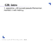
\onlySlide*{1}{1. spacetime = 4D (curved) pseudo-Riemannian manifold
$M$ with metric {\bf g}
\hypertarget{GRintro}{}
}
\fromSlide{2}{1. spacetime = 4D (curved) pseudo-Riemannian manifold
$M$ with metric {\bf g}
2. $\forall$ spacetime point $\mathbf{x}$
$\exists$ 4D Minkowski tangent space $T_{\mathbf{x}}M$ at $\mathbf{x}$}
\onlySlide*{3}{
= vector space (e.g. 4-momentum vectors)
}
\fromSlide{4}{
= vector space,
{\bf g}~$ \Rightarrow$ lengths of vectors in $T_{\mathbf{x}}M$
}
\fromSlide{5}{3. also, $\forall \mathbf{x} \in M,$
$\exists$ 4D Mink. cotangent space $T^*_{\mathbf{x}}M$}
\onlySlide*{6}{ = dual vector space (think: contour map, gradients)}
\fromSlide{7}{= space of one-forms, {\bf g}$^{-1} \Rightarrow$
``lengths"}
\onlySlide*{8}{duality in a basis of $T_{\mathbf{x}}M$ and a basis
of $T^*_{\mathbf{x}}M$ usually defined using $\delta^\mu_{\;\nu}$}
\fromSlide{9}{2+3. vector--one-form duality in a basis: $\delta^\mu_{\;\nu}$ }
\fromSlide{10}{4. \WikipediaEn{Levi-Civita connection} $\Leftarrow$ metric}
\fromSlide{11}{5. metric $\Leftarrow$ Einstein field equations}
\end{slide}
}
\parskip=12pt
\overlays{12}{%
\begin{slide}{GR: coordinate transformations}
\parskip=3pt %\small
\vspace{-5mm}
\onlySlide*{1}{
\begin{minipage}[b]{50mm}% width
\includegraphics[height=0.65\textheight]{Rotation_Euclidean1}
\hypertarget{coordtransf}{}
\end{minipage}
}
\onlySlide*{2}{
\begin{minipage}[b]{50mm}% width
\includegraphics[height=0.65\textheight]{Rotation_Euclidean2}
\end{minipage}
}
\fromSlide{3}{
\begin{minipage}[b]{50mm}% width
\includegraphics[height=0.65\textheight]{Rotation_Euclidean_basis}
\end{minipage}
}
\onlySlide*{3}{
\begin{minipage}[b]{50mm}% width
\vspace{50mm}
\end{minipage}
}
\onlySlide*{4}{
\begin{minipage}[b]{50mm}% width
$\left( \begin{array}{c} x' \\ y' \end{array} \right)
= \left( \begin{array}{cc}
\cos\theta & \sin\theta \\
-\sin\theta & \cos\theta
\end{array}
\right) \,
\left( \begin{array}{c} x \\ y \end{array} \right)
$ \\
\vspace{20mm}
\end{minipage}
}
\onlySlide*{5}{
\begin{minipage}[b]{50mm}% width
$\left( \begin{array}{c} x' \\ y' \end{array} \right)
= \Lambda \,
\left( \begin{array}{c} x \\ y \end{array} \right)
$ \\
\vspace{20mm}
\end{minipage}
}
\onlySlide*{6}{
\begin{minipage}[b]{50mm}% width
but
$\left( \begin{array}{c} \cos\theta \\ \sin\theta \end{array} \right)
= {
\left( \begin{array}{cc}
{ \cos\theta} & -\sin\theta \\
\sin\theta & \cos\theta
\end{array}
\right) \,
}
\left( \begin{array}{c} 1 \\ 0 \end{array} \right) $
\vspace{20mm}
\end{minipage}
}
\onlySlide*{7}{
\begin{minipage}[b]{50mm}% width
$\left( \begin{array}{c} \cos\theta \\ \sin\theta \end{array} \right)
= {\color{gray}
\left( \begin{array}{cc}
{\color{black} \cos\theta} & -\sin\theta \\
\sin\theta & \cos\theta
\end{array}
\right) \,
}
\left( \begin{array}{c} 1 \\ 0 \end{array} \right) + $
${\color{gray}
\left( \begin{array}{cc}
{\cos\theta} & -\sin\theta \\
{\color{black} \sin\theta} & \cos\theta
\end{array}
\right) \,
}
\left( \begin{array}{c} 0 \\ 1 \end{array} \right)
$ \\
\vspace{20mm}
\end{minipage}
}
\onlySlide*{8}{
\begin{minipage}[b]{50mm}% width
$ \vec{e}_{x'}
= {\color{gray} \left( \begin{array}{cc}
{\color{black} \cos\theta} & -\sin\theta \\
\sin\theta & \cos\theta
\end{array}
\right)} \,
\vec{e}_{x} + $
${\color{gray} \left( \begin{array}{cc}
{ \cos\theta} & -\sin\theta \\
{ \color{black} \sin\theta} & \cos\theta
\end{array}
\right)} \,
\vec{e}_{y}
$ \\
\vspace{10mm}
\end{minipage}
}
\onlySlide*{9}{
\begin{minipage}[b]{45mm}% width
$ \vec{e}_{x'}
= \Lambda^x_{x'} \,
\vec{e}_{x} + \Lambda^y_{x'} \,
\vec{e}_{y}
$ \\
\vspace{40mm}
\end{minipage}
}
\onlySlide*{10}{
\begin{minipage}[b]{45mm}% width
also: \\
$\left( \begin{array}{c} -\sin\theta \\ \cos\theta \end{array} \right)
= {\color{gray} \left(
\begin{array}{cc}
\cos\theta & {\color{black} -\sin\theta} \\
\sin\theta & \cos\theta
\end{array}
\right)} \,
\left( \begin{array}{c} 1 \\ 0 \end{array} \right) + $
$ {\color{gray} \left(
\begin{array}{cc}
\cos\theta & { -\sin\theta} \\
\sin\theta & {\color{black} \cos\theta }
\end{array}
\right)} \,
\left( \begin{array}{c} 0 \\ 1 \end{array} \right)
$ \\
\vspace{10mm}
\end{minipage}
}
\onlySlide*{11}{
\begin{minipage}[b]{45mm}% width
$ \vec{e}_{y'}
= {\color{gray} \left( \begin{array}{cc}
\cos\theta & {\color{black} -\sin\theta} \\
\sin\theta & \cos\theta
\end{array}
\right)} \,
\vec{e}_{x} + $
$ {\color{gray} \left( \begin{array}{cc}
\cos\theta & { -\sin\theta} \\
\sin\theta & {\color{black} \cos\theta }
\end{array}
\right)} \,
\vec{e}_{y}
$
\\ \vspace{10mm}
\end{minipage}
}
\fromSlide{12}{
\begin{minipage}[b]{45mm}% width
summary: \\
$ \vec{e}_{x'}
= \Lambda^x_{x'} \, \vec{e}_{x} +
\Lambda^y_{x'} \, \vec{e}_{y},
$ \\
$ \vec{e}_{y'}
= \Lambda^x_{y'} \, \vec{e}_{x} +
\Lambda^y_{y'} \, \vec{e}_{y} ,
$ \\
where $\Lambda^\alpha_{\beta'} :=$ element of
inverse of $\Lambda^{\alpha'}_{\beta}$,
\\
$\left( \begin{array}{c} x' \\ y' \end{array} \right)
= \Lambda \,
\left( \begin{array}{c} x \\ y \end{array} \right)
$
% \\ \vspace{10mm}
\end{minipage}
}
\end{slide}
}
\parskip=12pt
\overlays{10}{%
\begin{slide}{GR: coordinate transformations}
\parskip=4pt %\small
\vspace{-5mm}
\fromSlide{1}{
\begin{minipage}[b]{45mm}% width
$ \vec{e}_{x'}
= \Lambda^x_{x'} \, \vec{e}_{x} +
\Lambda^y_{x'} \, \vec{e}_{y},
$ \\
$ \vec{e}_{y'}
= \Lambda^x_{y'} \, \vec{e}_{x} +
\Lambda^y_{y'} \, \vec{e}_{y} ,
$
\end{minipage}
\begin{minipage}[b]{50mm}% width
$
\vec{p} \rightarrow_{{\cal O'}}
\left( \begin{array}{c} x' \\ y' \end{array} \right)
= \Lambda \,
\left( \begin{array}{c} x \\ y \end{array} \right)
$
\end{minipage}
}
\onlySlide*{2}{
$\vec{p} = \sum_i p^i \vec{e}_i $
}
\fromSlide{3}{
$\vec{p} = p^i \vec{e}_i $ (\WikipediaEn{Einstein summation})
}
\onlySlide*{4}{
Einstein summation: \hypertarget{summation}{}
$\bullet$ {{\bf coordinates} like $r,\theta,x,y$:
{\color{red} not a sum:}
$\Lambda^x_{y'} \, \vec{e}_{x}$}
$\bullet$ {repeated up-down coordinate
{\bf indices} like $i,j \in \{0,1,2\}$ or
$\alpha,\beta,\gamma,\lambda,\mu,\nu \in \{0,1,2,3\}$:
{\color{mygreen} sum:}
$\Lambda^i_{j'} \, \vec{e}_{i} :=
\Lambda^x_{y'} \, \vec{e}_{x} +
\Lambda^y_{y'} \, \vec{e}_{y}$ for a 2D manifold, coords $x,y$
}
}
\fromSlide{5}{
new basis vectors = sum of inverse $\Lambda \times$ {\color{red} old} vectors
}
\onlySlide*{6}{
$\vec{e}_{\mu'}
=
\sum_\nu \Lambda^\nu_{\;\mu'} \vec{e}_{\nu}
$}
\onlySlide*{7}{
$\vec{e}_{\mu'}
=
\Lambda^{\nu}_{\;\mu'}
\vec{e}_{\nu}
$}
\onlySlide*{8}{
new coords of vector $\vec{p}$ =
$\Lambda \times$ old coords of {\color{red} same} vector $\vec{p}$
}
\fromSlide{9}{
vector invariance requires contravariance of its coords\\
``contra" = inverse of change of basis vectors
}
\fromSlide{10}{
$\bullet$ $\vec{p}$ is invariant: no dependence on coords \\
$\bullet$ $\vec{p}$ is contravariant: $p^i$ change inversely to $\vec{e}_i$
}
% \fromSlide{11}{
\end{slide}
}
\parskip=12pt
\overlays{13}{%
\begin{slide}{GR: coord. transf.: 1-forms}
\parskip=1pt %\small
\vspace{-5mm}
\onlySlide*{1}{
$\phi$ = scalar field = $\phi(x,y) \equiv \phi(x',y')$
write $\phi_{,x} := \frac{\partial \phi}{\partial x}
=: (\tilde{\mathrm{d}} \phi)_x $
\hypertarget{scalarfield}{}
}
\fromSlide{2}{
$\phi$ = scalar field = $\phi(x,y) \equiv \phi(x',y')$
write $\phi_{,x} := \frac{\partial \phi}{\partial x}
=: (\tilde{\mathrm{d}} \phi)_x $
}
\onlySlide*{2}{
What is the relation between
$\left( \phi_{,x'} , \phi_{,y'} \right)$
and
$\left( \phi_{,x} , \phi_{,y} \right)$?
}
\onlySlide*{3}{
$\phi$ depends either on $x$ and $y$, or on $x'$ and $y'$
$\Rightarrow$ $\frac{\partial \phi}{\partial x'}
=
\frac{\partial \phi}{\partial x}
\frac{\partial x}{\partial x'}
+
\frac{\partial \phi}{\partial y}
\frac{\partial y}{\partial x'}
$
}
\fromSlide{4}{
$\phi$ depends either on $x$ and $y$, or on $x'$ and $y'$
$\Rightarrow$ $\phi_{,x'}
=
\phi_{,x} \,x_{,x'}
+
\phi_{,y} \,y_{,x'}
$
}
\fromSlide{5}{
$\left( \phi_{,x'} , \phi_{,y'} \right)
=$
}
\onlySlide*{6}{
$\left(
\phi_{,x} \, x_{,x'} + \phi_{,y} \,y_{,x'} \,,\,
\phi_{,x} \, x_{,y'} + \phi_{,y} \,y_{,y'}
\right)
$
}
\fromSlide{7}{
$
\left( \phi_{,x} , \phi_{,y} \right)
\left(
\begin{array}{cc}
x_{,x'} & x_{,y'} \\
y_{,x'} & y_{,y'}
\end{array}
\right)
$
}
\onlySlide*{8}{
$\left( \begin{array}{c} x \\ y \end{array} \right)
= \left( \begin{array}{cc}
\cos\theta & -\sin\theta \\
\sin\theta & \cos\theta
\end{array}
\right) \,
\left( \begin{array}{c} x' \\ y' \end{array} \right)
$ \quad (example: rotation)
$x_{,x'} = \frac{\partial x}{\partial x'} = \cos\theta $
$x_{,y'} = \frac{\partial x}{\partial y'} = -\sin\theta $
\ldots
}
\onlySlide*{9}{
$\left( \begin{array}{c} x \\ y \end{array} \right)
= \left( \begin{array}{cc}
x_{,x'} & x_{,y'} \\
y_{,x'} & y_{,y'}
\end{array}
\right) \,
\left( \begin{array}{c} x' \\ y' \end{array} \right)
$ \quad (general)
}
\fromSlide{10}{
$\left( \begin{array}{c} x \\ y \end{array} \right)
= \Lambda^{-1} \,
\left( \begin{array}{c} x' \\ y' \end{array} \right)
$ \quad (general)
}
\onlySlide*{11}{
$\Rightarrow$
$\left( \phi_{,x'} , \phi_{,y'} \right)
= \left( \phi_{,x} , \phi_{,y} \right) \Lambda^{-1}
$
}
\fromSlide{12}{
$\tilde{\mathrm{d}} \phi =
\left( (\tilde{\mathrm{d}} \phi)_{x'} , (\tilde{\mathrm{d}} \phi)_{y'} \right)
=
\left( (\tilde{\mathrm{d}} \phi)_x , (\tilde{\mathrm{d}} \phi)_y \right)
\Lambda^{-1}
$
}
\fromSlide{13}{
$(\tilde{\mathrm{d}}\phi)_{\mu'}
=
(\tilde{\mathrm{d}}\phi)_{\nu}
\Lambda^{\nu}_{\;\mu'}
$
}
\end{slide}
}
\parskip=12pt
\overlays{6}{%
\begin{slide}{GR: coord. transf.: 1-forms}
\parskip=1pt %\small
\vspace{-10mm}
\fromSlide{1}{
basis vectors of different bases: $\vec{e}_{\mu'}
=
%(\Lambda^{-1})^{\nu}_{\;\mu'}
\Lambda^{\nu}_{\;\mu'}
\vec{e}_{\nu}
$
}
\onlySlide*{1}{
same vector: $(\vec{p})^{\mu'}
=
\Lambda^{\mu'}_{\;\nu}
(\vec{p})^{\nu}
$
}
\fromSlide{2}{
same vector: $p^{\mu'}
=
\Lambda^{\mu'}_{\;\nu}
p^{\nu}
$
}
\fromSlide{1}{
same gradient (example 1-form): $(\tilde{\mathrm{d}}\phi)_{\mu'}
=
(\tilde{\mathrm{d}}\phi)_{\nu}
%(\Lambda^{-1})^{\nu}_{\;\mu'}
\Lambda^{\nu}_{\;\mu'}
$
}
\fromSlide{3}{
$\bullet$ vector $\vec{p}$ is {\color{blue} in}variant: no dependence on coords \\
$\bullet$ $\vec{p}$ is {\color{red} contra}variant:
components $p^\nu$ change inversely to how $\vec{e}_\mu$ change;
\quad inverses: matrix
$\{ \Lambda^{\nu}_{\;\mu'} \}$ vs $\{ \Lambda^{\beta'}_{\;\alpha} \}$
}
\fromSlide{4}{
$\bullet$ 1-form $\tilde{\mathrm{d}}\phi$ is {\color{blue} in}variant: no dependence on coords \\
$\bullet$ $\tilde{\mathrm{d}}\phi$ is {\color{mygreen} co}variant:
components $(\tilde{\mathrm{d}}\phi)_\mu$ change like $\vec{e}_\mu$
(but left-multiply)
}
\fromSlide{5}{
\WikipediaEn{Covariance and contravariance of vectors}
}
\fromSlide{6}{
{\color{red} Warning: common physics informal usage (but not this course!):
``covariant'' $:=$ ``invariant''}
}
\end{slide}
}
\overlays{13}{%
\begin{slide}{GR: $\vec{p}, \tilde{q}, \left< \vec{p}, \tilde{q} \right>,$
{\bf g}}
\parskip=7pt
\onlySlide*{1}{GR tensors: two different scalar products
\hypertarget{scalarprod}{}
}
\fromSlide{2}{GR tensors: two different scalar products}
\fromSlide{2}{
vector--1-form duality requirement:
}
\onlySlide*{3}{
$\left< \vec{p}, \tilde{q} \right> = \sum_\mu p^\mu q_\mu $
}
\onlySlide*{4}{
$\left< \vec{p}, \tilde{q} \right> = p^\mu q_\mu $
}
\onlySlide*{5}{
$\left< \vec{p}, \tilde{q} \right> = p^\mu q_\mu
= \vec{p}( \tilde{q}) $
}
\fromSlide{6}{
$\left< \vec{p}, \tilde{q} \right> = p^\mu q_\mu
= \vec{p}( \tilde{q})
= \tilde{q}(\vec{p} )
$
}
\fromSlide{7}{
$\left< \; ,\; \right>$ is a (1,1) tensor
}
\onlySlide*{8}{can be called $I$ with components $\delta^\mu_{\;\nu}$
in a coordinate basis}
\onlySlide*{9}{think: vector $\rightarrow$ column vector\\
1-form $\rightarrow$ row vector}
\fromSlide{10}{
$
( q_0 , q_1 )
\left( \begin{array}{cc} 1 & 0 \\ 0 & 1 \end{array} \right)
\left( \begin{array}{c} p^0 \\ p^1 \end{array} \right)
= $}
\fromSlide{11}{
$
( q_0 , q_1 )
\left( \begin{array}{c} p^0 \\ p^1 \end{array} \right)
$}
\fromSlide{12}{
$= p^\mu q_\mu $
}
\fromSlide{13}{$\left< \; ,\; \right>$ = (1,1)-tensor
= ``row-column" matrix $I$ with $I^\mu_{\;\nu} = \delta^\mu_{\;\nu}$}
\end{slide}
}
\overlays{14}{%
\begin{slide}{GR: $\vec{p}, \tilde{q}, \left< \vec{p}, \tilde{q} \right>,$
{\bf g}}
\vspace{-10mm}
\parskip=6pt
\fromSlide{1}{GR tensors: two different scalar products
}
\onlySlide*{2}{ordinary linear algebra: column vectors, row vectors,
matrices}
\fromSlide{3}{$(m,n)$-tensor algebra: $m$ column $n$ row $m+n$-arrays}
\onlySlide*{4}{e.g.: $(0,2)$-tensor: metric $g_{\mu\nu}$}
\onlySlide*{5}{using $\left<\;,\;\right>$, $(1,0)$-tensor =
vector = function of 1-forms}
\onlySlide*{6}{using $\left<\;,\;\right>$, $(0,1)$-tensor
= 1-form = function of vectors}
\fromSlide{7}{$(m,n)$-tensor = function of $m$ 1-forms and $n$ vectors}
\fromSlide{8}{$V=$ space of vectors $\vec{p} = p^\mu \vec{e}_\mu$}
\fromSlide{9}{$V^*=$ dual space of 1-forms $\tilde{q} = q_\mu \tilde{e}^\mu$}
\fromSlide{10}{$V^* \otimes V^*$ = space of $(0,2)$-tensors
{\bf T}~$= T_{\mu\nu} \tilde{e}^\mu \otimes \tilde{e}^\nu$ (e.g. metric)
\WikipediaEn{tensor product}}
\onlySlide*{11}{loosely speaking, the second $\otimes$ means
``function of two vectors" (or 1-forms, or a vector and a 1-form)
in {\em that particular left-to-right order}}
\fromSlide{12}{order of $V^* \otimes V^*$ = 2}
\onlySlide*{13}{{\color{red}warning: the ``rank" of tensors has two different meanings:}
\WikipediaEn{Tensor\_(intrinsic\_definition)\#Tensor\_rank}}
\fromSlide{14}{dimension of $V^* \otimes V^*$ = 16 (for $V=$ spacetime)}
\end{slide}
}
\overlays{18}{%
\begin{slide}{GR:
{\bf g}}
\parskip=5pt
\vspace{-10mm}
\onlySlide*{1}{$V^* \otimes V^*$ = space of $(0,2)$-tensors
{\bf T}~$ = T_{\mu\nu} \tilde{e}^\mu \otimes \tilde{e}^\nu$,
where $\otimes =$ \WikipediaEn{tensor product}
\hypertarget{metric}{}
}
\fromSlide{2}{$V^* \otimes V^*$ = space of $(0,2)$-tensors
$T = T_{\mu\nu} \tilde{e}^\mu \otimes \tilde{e}^\nu$,
where $\otimes =$ \WikipediaEn{tensor product}
}
\fromSlide{2}{e.g.:
metric {\bf g} = function of two vectors}
\fromSlide{3}{= ``row-row" matrix}
\fromSlide{4}{e.g. Euclidean {\bf g} on $\mathbb{R}^2$. \quad
{\bf g} in ${r,\theta}$ coords is
$\left( \begin{array}{cc} 1 & 0 \\ 0 & r^2 \end{array} \right)$
}
\fromSlide{5}{and {\bf g} in ${x,y}$ coords is
$\left( \begin{array}{cc} 1 & 0 \\ 0 & 1 \end{array} \right)$
\hypertarget{euclideanmetricR2}{}
}
\onlySlide*{6}{{\bf g}$(\vec{A},\vec{B})$}
\onlySlide*{7}{also written: $\vec{A} \cdot \vec{B}$ \quad ``dot product"}
\fromSlide{8}{{\bf g}$(\vec{A},\vec{B})$}
\onlySlide*{9}{$=
\left[
\left( \begin{array}{cc} 1 & 0 \\ 0 & r^2 \end{array} \right)
\left( \begin{array}{c} A^r \\ A^\theta \end{array} \right)
\right]\TTT
\left( \begin{array}{c} B^r \\ B^\theta \end{array} \right)
$}
\onlySlide*{10}{$=
\left( A^r , A^\theta r^2 \right)
\left( \begin{array}{c} B^r \\ B^\theta \end{array} \right)
$}
\fromSlide{11}{$=
A^r B^r + A^\theta B^\theta r^2
$}
\onlySlide*{12}{$=
\left[
\left( \begin{array}{cc} 1 & 0 \\ 0 & 1 \end{array} \right)
\left( \begin{array}{c} A^x \\ A^y \end{array} \right)
\right]\TTT
\left( \begin{array}{c} B^x \\ B^y \end{array} \right)
$}
\onlySlide*{13}{$=
\left( A^x , A^y \right)
\left( \begin{array}{c} B^x \\ B^y \end{array} \right)
$}
\fromSlide{14}{$=
A^x B^x + A^y B^y
$}
\onlySlide*{15}{in general, for a 2-form {\bf T},
{\bf T}$(\vec{A},\vec{B}) \not=
${\bf T}$(\vec{B},\vec{A})$}
\onlySlide*{16}{
{\bf g}~$= g_{\mu\nu} \tilde{e}^\mu \otimes \tilde{e}^\nu$
}
\onlySlide*{17}{
{\bf g}~$= \sum_{\mu \in \{r,\theta\}, \nu \in \{r,\theta\}}
g_{\mu\nu} \tilde{e}^\mu \otimes \tilde{e}^\nu$
}
\fromSlide{18}{
{\bf g}~$= \sum_{\mu \in \{x,y\}, \nu \in \{x,y\}}
g_{\mu\nu} \tilde{e}^\mu \otimes \tilde{e}^\nu$
}
\end{slide}
}
\overlays{20}{%
\begin{slide}{GR: metric tensor {\bf g},
%inverse metric tensor,
{\bf g}$^{-1}$,
bases
}
\parskip=6pt
\vspace{-10mm}
\fromSlide{1}{
{\bf g}$ $ can be applied to basis vectors
$\vec{e}_\mu$}
\fromSlide{2}{we can define components (used earlier):
$g_{\mu\nu} :=
$~{\bf g}$(\vec{e}_\mu, \vec{e}_\nu)$
}
\fromSlide{3}{$\Rightarrow$
{\bf g}~$ = g_{\mu\nu} \tilde{e}^\mu \otimes \tilde{e}^\nu$}
\onlySlide*{4}{e.g.
{\bf g}~$ =
g_{rr} \tilde{e}^r \otimes \tilde{e}^r +
g_{r\theta} \tilde{e}^r \otimes \tilde{e}^\theta +
g_{\theta r} \tilde{e}^\theta \otimes \tilde{e}^r +
g_{\theta\theta} \tilde{e}^\theta \otimes \tilde{e}^\theta
$}
\fromSlide{5}{e.g.
{\bf g}~$ =
g_{rr} \tilde{e}^r \otimes \tilde{e}^r +
g_{\theta\theta} \tilde{e}^\theta \otimes \tilde{e}^\theta
$}
\onlySlide*{6}{check:
{\bf g}$(\vec{e}_r, \vec{e}_r) = g_{rr} $?
}
\onlySlide*{7}{
{\bf g}$(\vec{e}_r, \vec{e}_r)
= (g_{rr} \tilde{e}^r \otimes \tilde{e}^r +
g_{\theta\theta} \tilde{e}^\theta \otimes \tilde{e}^\theta )
(\vec{e}_r, \vec{e}_r)$
}
\onlySlide*{8}{
{\bf g}$(\vec{e}_r, \vec{e}_r) = g_{rr} \tilde{e}^r \otimes \tilde{e}^r(\vec{e}_r, \vec{e}_r) +
g_{\theta\theta} \tilde{e}^\theta \otimes \tilde{e}^\theta
(\vec{e}_r, \vec{e}_r)
$
}
\onlySlide*{9}{
{\bf g}$(\vec{e}_r, \vec{e}_r) = g_{rr}\, \tilde{e}^r (\vec{e}_r)\, \tilde{e}^r (\vec{e}_r) +
g_{\theta\theta}\, \tilde{e}^\theta (\vec{e}_r)\, \tilde{e}^\theta (\vec{e}_r)
$
}
\onlySlide*{10}{
{\bf g}$(\vec{e}_r, \vec{e}_r) = g_{rr} \left<\tilde{e}^r ,\vec{e}_r\right>
\left< \tilde{e}^r , \vec{e}_r \right> +
g_{\theta\theta} \left<\tilde{e}^\theta ,\vec{e}_r\right>
\left< \tilde{e}^\theta, \vec{e}_r \right>
$
}
\onlySlide*{11}{
{\bf g}$(\vec{e}_r, \vec{e}_r) = g_{rr} \times 1 \times 1 +
g_{\theta\theta} \times 0 \times 0
$ by duality through scalar product $\left<\; , \;\right>$
}
\onlySlide*{12}{
{\bf g}$(\vec{e}_r, \vec{e}_r) = g_{rr} $ self-consistent definition
}
\fromSlide{13}{inverse:
{\bf g}$^{-1} =
g^{\mu\nu} \vec{e}_\mu \otimes \vec{e}_\nu$,
}
\fromSlide{14}{where
$g^{\mu\alpha}g_{\alpha\nu} = \delta^{\mu}_{\;\nu}$}
\fromSlide{15}{duality of associate vectors and 1-forms:}
\onlySlide*{15}{
{\bf g}$(\vec{A},\vec{B}) = $~{\bf g}$^{-1}(\tilde{A},\tilde{B})$
}
\onlySlide*{16}{{\bf g}$(\vec{A},\vec{B}) = $~{\bf g}$^{-1}(\tilde{A},\tilde{B})
= \vec{A} \cdot \vec{B} $}
\onlySlide*{17}{{\bf g}$(\vec{A},\vec{B}) = $~{\bf g}$^{-1}(\tilde{A},\tilde{B})
= \vec{A} \cdot \vec{B} = g_{\mu\nu} A^\mu B^\nu $}
\fromSlide{18}{\fbox{{\bf g}$(\vec{A},\vec{B}) = $~{\bf g}$^{-1}(\tilde{A},\tilde{B})
= \vec{A} \cdot \vec{B} = g_{\mu\nu} A^\mu B^\nu= g^{\mu\nu} A_\mu B_\nu $}}
\onlySlide*{19}{
\fbox{lower an index: $g_{\mu\nu} A^\mu = A_\nu$}}
\fromSlide{20}{
\fbox{lower index: $g_{\mu\nu} A^\mu = A_\nu$}\,
\fbox{raise index: $g^{\mu\nu} B_\nu = B^\mu$}}
\end{slide}
}
\overlays{9}{%
\begin{slide}{GR: what is a coordinate?
}
\parskip=6pt
\vspace{-10mm}
\onlySlide*{1}{a coordinate, e.g. $x^0$ or $x^1$ is
a scalar field on the 4-manifold
\hypertarget{coordinate}{}
}
\fromSlide{2}{a coordinate system $x^\mu$ = set of four
scalar fields
on the 4-manifold}
\onlySlide*{3}{(Bertschinger writes $x^\mu_{\mathbf{x}}$
to show dependence
on position $\mathbf{x}$ in manifold $\not=$ vector space)}
\fromSlide{4}{$x^\mu$ are differentiable {\em almost everywhere}}
\onlySlide*{5}{\includegraphics[height=0.55\textheight]{Scalar_fields_x}
e.g. on $\mathbb{R}^2$}
\onlySlide*{6}{\includegraphics[height=0.55\textheight]{Scalar_fields_y}
e.g. on $\mathbb{R}^2$}
\onlySlide*{7}{\includegraphics[height=0.55\textheight]{Scalar_fields_r}
e.g. on $\mathbb{R}^2$}
\fromSlide{8}{\includegraphics[height=0.55\textheight]{Scalar_fields_theta}
e.g. on $\mathbb{R}^2$}
\fromSlide{9}{coordinate singularity $\not=$ singularity in manifold}
\end{slide}
}
}
\GRslides{
\overlays{13}{%
\begin{slide}{GR: what is a coordinate basis?}
\parskip=2pt
\vspace{-10mm}
\fromSlide{1}{coordinate basis: $\vec{e}_\mu$, $\tilde{e}^\nu$ chosen so that:
$\mathrm{d}\vec{x} = \mathrm{d}x^\mu \vec{e}_\mu$ and}
\fromSlide{2}{
{\color{mygreen}
$\mathrm{d}f = \left< \tilde{\mathrm{d}}f, \mathrm{d}\vec{x}\right>$} for any scalar field
$f$ {\color{mygreen} coordinate-free}
where $\tilde{\mathrm{d}} = \tilde{e}^\mu \partial_\mu$ in a coordinate basis}
\onlySlide*{3}{(Bertschinger writes $\widetilde{\nabla}$ for the gradient $\tilde{\mathrm{d}}$)}
\fromSlide{4}{check:
$\mathrm{d}f = \left< \tilde{\mathrm{d}}f, \mathrm{d}\vec{x}\right>$ }
\fromSlide{5}{$=\left< \tilde{e}^\mu \partial_\mu f, \mathrm{d}x^\nu \vec{e}_\nu\right>$ }
\fromSlide{6}{$=(\partial_\mu f) \, \mathrm{d}x^\nu \left< \tilde{e}^\mu , \vec{e}_\nu\right>$ since scalars commute}
\onlySlide*{7}{i.e. $\mathrm{d}f= (\partial_\mu f) \, \mathrm{d}x^\mu $ since $\left< \tilde{e}^\mu , \vec{e}_\nu\right> = \delta^\mu_\nu$}
\onlySlide*{8}{i.e. $\mathrm{d}f = \sum_\mu \frac{\partial f}{\partial x^\mu} \, \mathrm{d}x^\mu $}
\fromSlide{9}{i.e. $\mathrm{d}f=(\partial_\mu f) \, \mathrm{d}x^\mu $}
\fromSlide{10}{check:
$\tilde{\mathrm{d}} x^\mu = \tilde{e}^\nu \partial_\nu x^\mu $
}
\onlySlide*{11}{$ = \sum_\nu \tilde{e}^\nu \partial_\nu x^\mu $}
\onlySlide*{12}{$ = \sum_\nu \tilde{e}^\nu \frac{\partial}{\partial x^\nu} x^\mu $}
\fromSlide{13}{$ = \tilde{e}^\mu $}
\end{slide}
}
\overlays{5}{%
\begin{slide}{GR: metric using $\mathrm{d}\vec{x}$
}
\parskip=6pt
% \vspace{-10mm}
\onlySlide*{1}{we now have \hypertarget{dstwo}{}}
\fromSlide{2}{we now have }
\onlySlide*{2}{$\mathrm{d}s^2 := |\mathrm{d}\vec{x} |^2$}
\onlySlide*{3}{$\mathrm{d}s^2 := |\mathrm{d}\vec{x} |^2
:= ${\bf g}$(\mathrm{d}\vec{x},\mathrm{d}\vec{x})$}
\fromSlide{4}{
{\color{mygreen}
$\mathrm{d}s^2 := |\mathrm{d}\vec{x} |^2
:= ${\bf g}$(\mathrm{d}\vec{x},\mathrm{d}\vec{x})
= \mathrm{d}\vec{x} \cdot \mathrm{d}\vec{x}
$ coordinate-free}}
\fromSlide{5}{
$\mathrm{d}s^2 = g_{\mu\nu} \mathrm{d}x^\mu \mathrm{d} x^\nu$
if $x^\mu$ are a coordinate basis}
\end{slide}
}
\overlays{7}{%
\begin{slide}{GR: e.g. Euclidean {\bf g} on $\mathbb{R}^2$}
\parskip=2pt
\vspace{-10mm}
\fromSlide{1}{
\hyperlink{euclideanmetricR2}{$g_{r\theta}$ and $g_{xy}$}
$\mathrm{d}s^2 = \mathrm{d}x^2 + \mathrm{d}y^2
= \mathrm{d}r^2 + r^2 \mathrm{d}\theta^2$
}
\fromSlide{2}{
$\vec{e}_x \cdot \vec{e}_x = 1 = \vec{e}_y \cdot \vec{e}_y$, others zero
}
\fromSlide{3}{
$\vec{e}_r \cdot \vec{e}_r = 1$, $\vec{e}_\theta \cdot \vec{e}_\theta = r^2 \not= 1$
}
\onlySlide*{3}{
\includegraphics[height=0.55\textheight]{Vector_basis_polar_coordinates}}
\fromSlide{4}{
$g^{\mu\alpha}g_{\alpha\nu} = \delta^{\mu}_{\;\nu}$
$\Rightarrow$
$g^{xx} = 1 = g^{yy}, g^{xy} = 0 = g^{yx}$}
\fromSlide{5}{
but $g^{rr} = 1 \not= g^{\theta\theta} = r^{-2}, g^{r\theta} = 0 = g^{\theta r}$}
\fromSlide{6}{
\includegraphics[height=0.50\textheight]{One-form_basis_polar_coordinates}}
\fromSlide{7}{
so $\tilde{e}^r \cdot \tilde{e}^r = 1$, $\tilde{e}^\theta \cdot \tilde{e}^\theta = r^{-2} \not= 1$
}
\end{slide}
}
\parskip=12pt
\overlays{14}{%
\begin{slide}{GR: gradient of a vector: $\nabla\vec{A}$}
% \WikipediaEn{Intermediate treatment of tensors}
\parskip=3pt
\vspace{-10mm}
\onlySlide*{1}{\hyperlink{scalarfield}{gradient of scalar field}:
$\tilde{\mathrm{d}}\phi \equiv \widetilde{\nabla}\phi$
\hypertarget{gradvec}{}}
\onlySlide*{2}{what is gradient of vector field
$\widetilde{\nabla}\vec{A}$?}
\fromSlide{3}{$\widetilde{\nabla}\vec{A} =
\widetilde{\nabla}(A^\nu \vec{e}_\nu) $}
\fromSlide{4}{$= \tilde{e}^\mu \partial_\mu (A^\nu \vec{e}_\nu) $}
\onlySlide*{5}{$= \tilde{e}^\mu \otimes
[(\partial_\mu A^\nu) \vec{e}_\nu
+ A^\nu \partial_\mu \vec{e}_\nu ]$ by product rule and linearity}
\fromSlide{6}{$= \partial_\mu A^\nu \tilde{e}^\mu \otimes \vec{e}_\nu
+
A^\nu \tilde{e}^\mu \otimes \partial_\mu \vec{e}_\nu$ }
\onlySlide*{7}{give a name to the second part: it must be a linear
combination of basis vectors $\vec{e}_\lambda$}
\fromSlide{8}{define $\Gamma^\lambda_{\; \nu\mu} \vec{e}_\lambda :=
\partial_\mu \vec{e}_\nu$
{\color{mygreen} Christoffel symbols of second kind (symmetric defn)}}
\fromSlide{9}{so $\widetilde{\nabla}\vec{A} =
\partial_\mu A^\nu \tilde{e}^\mu \otimes \vec{e}_\nu
+
A^\nu \tilde{e}^\mu \otimes \Gamma^\lambda_{\; \nu\mu} \vec{e}_\lambda$
}
\onlySlide*{10}{$=
\partial_\mu A^\nu \tilde{e}^\mu \otimes \vec{e}_\nu
+
A^\nu \Gamma^\lambda_{\; \nu\mu} \tilde{e}^\mu \otimes \vec{e}_\lambda
$ since any $\Gamma^\lambda_{\; \nu\mu}$ is a scalar}
\fromSlide{11}{$=
\partial_\mu A^\nu \tilde{e}^\mu \otimes \vec{e}_\nu
+
A^\lambda \Gamma^\nu_{\; \lambda\mu} \tilde{e}^\mu \otimes \vec{e}_\nu$
% A^\nu \Gamma^\lambda_{\; \nu\mu} \tilde{e}^\mu \otimes \vec{e}_\lambda
}
\onlySlide*{11}{since name of summation index is arbitrary, e.g.
$ \sum_\lambda x^{-2\lambda} = \sum_\mu x^{-2\mu} = \sum_\nu x^{-2\nu} $}
\fromSlide{12}{$=
(\partial_\mu A^\nu
+
A^\lambda \Gamma^\nu_{\; \lambda\mu}) \tilde{e}^\mu \otimes \vec{e}_\nu$
% A^\nu \Gamma^\lambda_{\; \nu\mu} \tilde{e}^\mu \otimes \vec{e}_\lambda
}
\onlySlide*{13}{
\begin{centering}
{\color{mygreen} \fbox{
$\nabla_\mu A^\nu := A^\nu_{\; ;\mu} :=
\partial_\mu A^\nu
+
A^\lambda \Gamma^\nu_{\; \lambda\mu}
$}
\WikipediaEn{covariant derivative} of vector}
\end{centering}
}
\fromSlide{14}{ \hypertarget{gradvecfinal}{}
\begin{centering}
{\color{mygreen} \fbox{
$\nabla_\mu A^\nu := A^\nu_{\; ;\mu} :=
A^\nu_{\; ,\mu}
+
A^\lambda \Gamma^\nu_{\; \lambda\mu}
$}
\WikipediaEn{covariant derivative} of vector}
\end{centering}
}
\end{slide}
}
\parskip=3pt
\overlays{9}{%
\begin{slide}{GR: $\widetilde{\nabla}$ and $\Gamma^\nu_{\;\lambda\mu}$}
\vspace{-8mm}
\fromSlide{1}{mathematically deeper: $\widetilde{\nabla}$, usually
written just as $\nabla$, is the
\WikipediaEn{Levi-Civita connection}}
\fromSlide{2}{{\color{red} warning: $\Gamma^\nu_{\;\lambda\mu}$
are NOT the components of a tensor}}
\fromSlide{3}{$\bullet$ $\widetilde{\nabla}$ applied to a $(m,n)$-tensor field
on a manifold gives an $(m,n+1)$-tensor field}
\onlySlide*{4}{so far we showed how $\widetilde{\nabla}$
applied to a $(0,0)$-tensor field = scalar field $\phi$
gives a $(0,1)$-tensor field = one-form field =
$(\tilde{\mathrm{d}} \phi)_\mu \tilde{e}^\mu$}
\fromSlide{5}{so far we showed how $\widetilde{\nabla}$
applied to a $(0,0)$-tensor field = scalar field $\phi$
gives a $(0,1)$-tensor field = one-form field =
$({\nabla}_\mu \phi) \tilde{e}^\mu
=(\partial_\mu \phi) \tilde{e}^\mu$}
\fromSlide{6}{and $\widetilde{\nabla}$
on a $(1,0)$-tensor field = vector field $\vec{A}$
gives a $(1,1)$-tensor with components
$\nabla_\mu A^\nu =
\partial_\mu A^\nu + A^\lambda \Gamma^\nu_{\; \lambda\mu}$
}
\fromSlide{7}{$\bullet$ tensors:
$\widetilde{\nabla}\phi = (\partial_\mu \phi) \tilde{e}^\mu$,
}
\fromSlide{8}{
$\; \widetilde{\nabla} \vec{A} =
\left(\partial_\mu A^\nu + A^\lambda \Gamma^\nu_{\; \lambda\mu}\right)
\tilde{e}^\mu \otimes \vec{e}_\nu$ }
\fromSlide{9}{
$\bullet$ not components of tensor: $\Gamma^\nu_{\; \lambda\mu}$
\hypertarget{Gammanottensor}{}
}
\end{slide}
}
\parskip=12pt
\overlays{18}{%
\begin{slide}{GR: gradient of one-form $\widetilde{\nabla}\tilde{A}$ }
% \WikipediaEn{Intermediate treatment of tensors}
\parskip=3pt
\vspace{-10mm}
\onlySlide*{1}{how does a one-form change with position? $\widetilde{\nabla}\tilde{A} =$?}
\fromSlide{2}{evaluating $\widetilde{\nabla}\tilde{A}$ as we did
$\widetilde{\nabla}\vec{A}$ shows that we again need
$\partial_\mu \tilde{e}^\nu = F^\nu_{\; \lambda\mu} \tilde{e}^\lambda$
for some coefficients $F^\nu_{\; \lambda\mu}$}
\fromSlide{3}{how can we relate $\Gamma^\nu_{\; \lambda\mu}$ to
$F^\nu_{\; \lambda\mu}$ ?}
\fromSlide{4}{
relation between vectors and one-forms:
$\left< \tilde{e}^\nu, \vec{e}_\lambda \right> = \delta^\nu_{\; \lambda}$
}
\onlySlide*{5}{
$ \partial_\mu \delta^\nu_{\; \lambda} = 0$ (obviously)}
\fromSlide{6}{
$ 0 = \partial_\mu \delta^\nu_{\; \lambda}
= \partial_\mu \left( \left< \tilde{e}^\nu, \vec{e}_\lambda \right> \right) $
}
\onlySlide*{7}{can we use the product rule with this scalar product?
$ \partial_\mu \left(\left< \tilde{A}, \vec{B} \right> \right) =$ ?
}
\onlySlide*{8}{can we use the product rule with this scalar product?
$ \partial_\mu \left(\left< \tilde{A}, \vec{B} \right> \right) =
\partial_\mu \left(A_\nu B^\nu \right)$ in some coordinate basis}
\onlySlide*{9}{can we use the product rule with this scalar product?
$ \partial_\mu \left(\left< \tilde{A}, \vec{B} \right> \right) =
\partial_\mu \left(A_\nu B^\nu \right)$
$=(\partial_\mu A_\nu) B^\nu + A_\nu (\partial_\mu B^\nu)$ by product rule
on functions}
\onlySlide*{10}{can we use the product rule with this scalar product?
$ \partial_\mu \left(\left< \tilde{A}, \vec{B} \right> \right) =
\partial_\mu \left(A_\nu B^\nu \right)$
$=(\partial_\mu A_\nu) B^\nu + A_\nu (\partial_\mu B^\nu)$
$=\left< \partial_\mu \tilde{A}, \vec{B} \right> +
\left< \tilde{A}, \partial_\mu \vec{B} \right>$
since $\partial_\mu \tilde{A} = \left( \partial_\mu A_0, \partial_\mu A_1, \partial_\mu A_2, \partial_\mu A_3 \right)$}
\fromSlide{11}{product rule holds:
$ \partial_\mu \left(\left< \tilde{A}, \vec{B} \right> \right) =
\left< \partial_\mu \tilde{A}, \vec{B} \right> +
\left< \tilde{A}, \partial_\mu \vec{B} \right>$
}
\fromSlide{12}{
so
$ 0 =
\left< \partial_\mu \tilde{e}^\nu, \vec{e}_\lambda \right> +
\left< \tilde{e}^\nu , \partial_\mu \vec{e}_\lambda \right> $}
\onlySlide*{13}{
$= \left< F^\nu_{\; \kappa\mu} \tilde{e}^\kappa, \vec{e}_\lambda \right>
+ \left< \tilde{e}^\nu , \Gamma^\kappa_{\; \lambda\mu} \vec{e}_\kappa \right>$}
\onlySlide*{14}{
$= F^\nu_{\; \kappa\mu} \left< \tilde{e}^\kappa, \vec{e}_\lambda \right>
+ \Gamma^\kappa_{\; \lambda\mu} \left< \tilde{e}^\nu , \vec{e}_\kappa \right>$}
\fromSlide{15}{
$= F^\nu_{\; \lambda\mu}
+ \Gamma^\nu_{\; \lambda\mu} $ since
$\left< \tilde{e}^\kappa, \vec{e}_\lambda \right> = \delta^\kappa_{\;\lambda}$ }
\fromSlide{16}{hence,
$\partial_\mu \tilde{e}^\nu =:
F^\nu_{\; \lambda\mu} \tilde{e}^\lambda
= -\Gamma^\nu_{\; \lambda\mu} \tilde{e}^\lambda$}
\onlySlide*{17}{
\fbox{
${\nabla}_\mu A^\nu = \partial_\mu A^\nu + A^\lambda \Gamma^\nu_{\; \lambda\mu}$
\quad , \quad
${\nabla}_\mu A_\nu = \partial_\mu A_\nu - A_\lambda \Gamma^\lambda_{\; \mu\nu}$
}
}
\fromSlide{18}{
\fbox{{\color{mygreen}
$A^\nu_{\;;\mu} = A^\nu_{\; ,\mu} + A^\lambda \Gamma^\nu_{\; \lambda\mu}$
\quad , \quad
$A_{\nu ; \mu} = A_{\nu , \mu} - A_\lambda \Gamma^\lambda_{\; \mu\nu}$
}
}}
\end{slide}
}
\parskip=12pt
\overlays{4}{%
\begin{slide}{GR: smooth manifold and $\widetilde{\nabla}${\bf g}}
\parskip=3pt %\small
\vspace{-10mm}
\fromSlide{1}{similarly, we can write the $(0,3)$-tensor
$\widetilde{\nabla} ${\bf g}~$ =
(\nabla_\lambda g_{\mu\nu}) \tilde{e}^\lambda \otimes
\tilde{e}^\mu \otimes \tilde{e}^\nu$
giving
$\nabla_\lambda g_{\mu\nu} =
\partial_\lambda g_{\mu\nu}
- \Gamma^\kappa_{\; \mu\lambda} g_{\kappa\nu}
- \Gamma^\kappa_{\; \nu\lambda} g_{\mu\kappa} $
}
\onlySlide*{1}{\hypertarget{manifold}{}}
\fromSlide{2}{also
$\widetilde{\nabla} ${\bf g}$^{-1} =
(\nabla_\lambda g^{\mu\nu}) \tilde{e}^\lambda \otimes
\vec{e}_\mu \otimes \vec{e}_\nu$
and
$\nabla_\lambda g^{\mu\nu} =
\partial_\lambda g^{\mu\nu}
+ \Gamma^\mu_{\; \kappa\lambda} g_{\kappa\nu}
+ \Gamma^\nu_{\; \kappa\lambda} g_{\mu\kappa} $}
\fromSlide{3}{
Do we know anything interesting about
$\widetilde{\nabla} ${\bf g}
for the manifolds of interest to GR?}
\fromSlide{4}{First, we need a rough description of
the manifolds we need for GR.}
% {\color{mygreen} at coordinate system
% if $\vec{e}_\mu \cdot \vec{e}_\nu = \pm \delta^\mu_\nu$
% in limit near a point $\forall \mu, \nu \in \{ 0, 1, 2, 3\}$}}
\end{slide}
}
}
\GRslides{
\parskip=12pt
\overlays{5}{%
\begin{slide}{GR: smooth manifold and $\widetilde{\nabla}${\bf g}}
\parskip=3pt %\small
\vspace{-10mm}
\fromSlide{1}{
{\color{mygreen} topological manifold $M$
\WikipediaEn{Manifold\#Mathematical\_definition}}
$\bullet$ only topological properties needed
}
\onlySlide*{2}{$\bullet$ no differentiability, no metric needed}
\fromSlide{3}{next: relation with $\mathbb{R}^4$ (or M$^4$)}
\fromSlide{4}{
\begin{minipage}[b]{55mm}
\includegraphics[height=0.5\textheight]{500px-Circle_with_overlapping_manifold_charts}
\WMCommons{Circle_with_overlapping_manifold_charts.svg}
\end{minipage}
}
% \WikipediaEnTwo{Manifold\#Charts.2C_atlases.2C_and_transition_maps}{Manifold\#Charts.2C\_atlases.2C\_and\_transition\_maps}
\fromSlide{5}{
\begin{minipage}[b]{50mm}
\WikipediaEnTwo{Manifold\#Charts.2C_atlases.2C_and_transition_maps}{Manifold}
$\bullet$ chart := function $\phi_\alpha$ from part of pseudo-4-manifold $M$ to part of M$^4$ (Minkowski)
$\bullet$ atlas := set of overlapping charts that cover $M$
\vspace{10mm}
\end{minipage}
}
\end{slide}
}
\newcommand\ifeverytransitionchart{
{\color{red}if} every transition chart $:= \phi_\beta \circ \phi_\alpha^{-1}$
%% \WikipediaEn{Function composition}
in an atlas for $M$ is
differentiable on $\mathbb{R}^4$ (or M$^4$), then
{\color{mygreen} $M$ is a
\WikipediaEnTwo{differentiable manifold}{differentiable 4-(pseudo-)manifold}}
}
\overlays{5}{%
\begin{slide}{GR: smooth manifold and $\widetilde{\nabla}${\bf g}}
\parskip=3pt %\small
\vspace{-11mm}
\fromSlide{1}{\ifeverytransitionchart}
\fromSlide{2}{
\includegraphics[height=0.6\textheight]{Nondifferentiable_atlas}
\WikipediaEnTwo{File:Nondifferentiable\_atlas.png}{}
}
\onlySlide*{3}{
projections (left-to-right) $\phi_1$, $\phi_2$, $\phi_3$ from $S^2$ to $\mathbb{R}^2$
}
\onlySlide*{4}{
$\phi_1$ is not differentiable, so $\phi_1 \circ \phi_2^{-1}$ is not differentiable
}
\fromSlide{5}{
atlas not enough to show that $S^2 =$ differentiable
2-manifold
}
\end{slide}
}
\overlays{4}{%
\begin{slide}{GR: smooth manifold and $\widetilde{\nabla}${\bf g}}
\parskip=3pt %\small
% \vspace{-10mm}
\fromSlide{1}{\ifeverytransitionchart}
\fromSlide{2}{{\color{red}if} $\forall k \ge 1$, $\exists k$-th derivatives,
then
{\color{mygreen} $M$ is a smooth 4-(pseudo-)manifold}}
\fromSlide{3}{{\color{red}if} a (pseudo-)\WikipediaEn{Riemannian metric} {\bf g} can be added to $M$,
then $(M,${\bf g}$)$ is a (pseudo-)Riemannian 4-manifold}
\fromSlide{4}{{\color{red}if} {\bf g} has signature $(1,n-1)$ (i.e. $(-,+,+,+)$ or $(+,-,-,-)$, etc.),
then $(M,${\bf g}$)$ is a Lorentzian $n$-manifold}
\end{slide}
}
\overlays{7}{%
\begin{slide}{GR: smooth manifold and $\widetilde{\nabla}${\bf g}}
\parskip=3pt %\small
% \vspace{-10mm}
\onlySlide*{1}{\fbox{\parbox{90mm}{
topological~manifolds}}
}
\onlySlide*{2}{\fbox{\parbox{90mm}{
\mbox{topological~manifolds}
\fbox{\parbox{85mm}{differentiable\ (pseudo-)manifolds}}
}}
}
\onlySlide*{3}{\fbox{\parbox{90mm}{
\mbox{topological\ manifolds}
\fbox{\parbox{85mm}{
\mbox{differentiable\ (pseudo-)manifolds}
\fbox{\parbox{80mm}{smooth\ (pseudo-)manifolds}}
}}
}}
}
\onlySlide*{4}{\fbox{\parbox{90mm}{
\mbox{topological\ manifolds}
\fbox{\parbox{85mm}{
\mbox{differentiable\ (pseudo-)manifolds}
\fbox{\parbox{80mm}{
\mbox{smooth\ (pseudo-)manifolds}
\fbox{\parbox{75mm}{(pseudo-)Riemannian\ manifolds}}
}}
}}
}}
}
\onlySlide*{5}{\fbox{\parbox{90mm}{
\mbox{topological\ manifolds}
\fbox{\parbox{85mm}{
\mbox{differentiable\ (pseudo-)manifolds}
\fbox{\parbox{80mm}{
\mbox{smooth\ (pseudo-)manifolds}
\fbox{\parbox{75mm}{
\mbox{(pseudo-)Riemannian\ manifolds}
\fbox{\parbox{70mm}{Lorentzian\ manifolds}}
}}
}}
}}
}}
}
\fromSlide{6}{\fbox{\parbox{90mm}{
\mbox{topological\ manifolds}
\fbox{\parbox{85mm}{
\mbox{differentiable\ (pseudo-)manifolds}
\fbox{\parbox{80mm}{
\mbox{smooth\ (pseudo-)manifolds}
\fbox{\parbox{75mm}{
\mbox{(pseudo-)Riemannian\ manifolds}
\fbox{\parbox{70mm}{
\mbox{Lorentzian\ manifolds}
\fbox{\parbox{65mm}{Lorentzian\ 4-manifolds}}
}}
}}
}}
}}
}}
}
\fromSlide{7}{\fbox{\color{mygreen} GR: assume that spacetime is a Lorentzian 4-manifold}}
\end{slide}
}
\parskip=12pt
\overlays{11}{%
\begin{slide}{GR: smooth manifold and $\widetilde{\nabla}${\bf g}}
\parskip=1pt %\small
\vspace{-10mm}
% {\color{mygreen} smooth pseudo-4-manifold $M$:
% $\forall$ point $\mathbf{x} \in M$,
% $\exists$ a locally flat coordinate system
% $\{\vec{e}^{\bar{\mu}}, \bar{\mu}=0,1,2,3\}$ at $\mathbf{x}$, i.e. where
% $g_{\bar{\mu}\bar{\nu}} =
% \vec{e}_{\bar{\mu}} \cdot \vec{e}_{\bar{\nu}} = \pm \delta^{\bar{\mu}}_{\bar{\nu}}$
% in limit of neighbourhood of
% $\mathbf{x}$}
\fromSlide{1}{from \hyperlink{manifold}{above}:
$\nabla_\lambda g_{\mu\nu} =
\partial_\lambda g_{\mu\nu}
- \Gamma^\kappa_{\; \mu\lambda} g_{\kappa\nu}
- \Gamma^\kappa_{\; \nu\lambda} g_{\mu\kappa} $
}
\fromSlide{2}{in the tangent space at $\mathbf{x},$ $\exists$
coordinate basis $\vec{e}_{\bar{\mu}}$ with
% $g_{\bar{i}\,\bar{j}} = \delta_{\bar{i}\,\bar{j}} = g^{\bar{i}\,\bar{j}}$
% for a 3-spatial slice
$g_{\bar{\mu}\bar{\nu}} = \eta_{\bar{\mu}\bar{\nu}} =
\mathrm{diag}(-1,1,1,1) = g^{\bar{\mu}\bar{\nu}}$}
\fromSlide{2}{$\Rightarrow$
$\partial_{\bar{\lambda}} g_{\bar{\mu}\bar{\nu}} =
\partial_{\bar{\lambda}} \eta_{\bar{\mu}\bar{\nu}}$
}
\fromSlide{3}{$= 0$}
\fromSlide{4}{also,
$\Gamma^{\bar{\lambda}}_{\; \bar{\nu}\bar{\mu}} \vec{e}_{\bar{\lambda}} :=
\vec{e}_{\bar{\nu},\bar{\mu}}
= \partial_{\bar{\mu}} \vec{e}_{\bar{\nu}}
$ }
\onlySlide*{5}{but in a Cartesian or Minkowski (vector) space, the
basis vectors always point in the same direction and their
lengths are fixed}
\onlySlide*{6}{M$^4$ $\Rightarrow$ $\Gamma^{\bar{\lambda}}_{\; \bar{\nu}\bar{\mu}} \vec{e}_{\bar{\lambda}} =0$}
\fromSlide{7}{so $\nabla_{\bar{\lambda}} g_{\bar{\mu}\bar{\nu}} = 0$}
\onlySlide*{8}{so $\widetilde{\nabla}${\bf g}~$ = \mathbf{0}$ (also $\widetilde{\nabla}${\bf g}$^{-1} =0$)
on the tangent space, since if true in one coord system, also true in others}
\fromSlide{9}{so $\widetilde{\nabla}${\bf g}~$ = \mathbf{0} = \widetilde{\nabla}${\bf g}$^{-1}$ on tangent space}
\fromSlide{9}{\ldots $\widetilde{\nabla}${\bf g}~$ = \mathbf{0} = \widetilde{\nabla}${\bf g}$^{-1}$ on $M$}
\fromSlide{10}{\ldots $\Gamma^\lambda_{\;\mu\nu} = \Gamma^\lambda_{\;\nu\mu}$
in any coord. basis (symmetric defn)}
\fromSlide{11}{\ldots
\fbox{{\color{mygreen} $\Gamma^\lambda_{\;\mu\nu} = \frac{1}{2}
g^{\lambda\kappa} (\partial_\mu g_{\nu\kappa}
+ \partial_\nu g_{\mu\kappa}
- \partial_\kappa g_{\mu\nu})$ in a coordinate basis}}
\hypertarget{Gammafrommetric}{}
}
\end{slide}
}
\parskip=12pt
\overlays{7}{%
\begin{slide}{GR: directional deriv.: $<\widetilde{\nabla}\vec{A}, \vec{V}>$ }
% \WikipediaEn{Intermediate treatment of tensors}
\parskip=3pt
\vspace{-10mm}
\fromSlide{1}{
$\bullet$ $\widetilde{\nabla}\phi,
\widetilde{\nabla}\vec{A},
\widetilde{\nabla}\tilde{A}$ gave how the fields $\phi$, $\vec{A}$,
or $\tilde{A}$ change around the manifold in general}
\onlySlide*{1}{\hypertarget{dirderiv}{}}
\fromSlide{2}{$\bullet$ how about moving along a specific curve?}
\fromSlide{3}{$\bullet$ curve on manifold parametrised by
a continuously changing real parameter $\lambda$:
$\mathbf{x}(\lambda)$ }
\fromSlide{4}{$ = \{x^\mu(\lambda)\}$ in a coordinate basis}
\fromSlide{5}{$\bullet$ can define tangent vectors along the
curve, i.e.
$\vec{V}(\lambda) := \frac{\mathrm{d}\vec{x}}{\mathrm{d}\lambda}$
}
\fromSlide{6}{$= \frac{\mathrm{d}x^\mu}{\mathrm{d}\lambda} \vec{e}_\mu$}
\fromSlide{7}{{\color{red} warning: $\{x^\mu(\lambda)\}$ at some $\lambda$
on the manifold is a point on the manifold but NOT a vector;
while $\mathrm{d}\vec{x}$ --- in the tangent space ---
IS a vector}}
\end{slide}
}
\overlays{12}{%
\begin{slide}{GR: directional deriv.: $<\widetilde{\nabla}\vec{A}, \vec{V}>$ }
% \WikipediaEn{Intermediate treatment of tensors}
\parskip=3pt
\vspace{-10mm}
\fromSlide{1}{
using $\vec{V}(\lambda) := \frac{\mathrm{d}\vec{x}}{\mathrm{d}\lambda}$,
project covariant derivative to curve using scalar product
$\left<\,,\,\right>$}
\fromSlide{2}{
$\frac{\mathrm{d}\phi}{\mathrm{d}\lambda} \equiv
\nabla_V \phi : = \left< \widetilde{\nabla}\phi, \vec{V} \right>$}
\onlySlide*{3}{or in a coordinate basis\ldots}
\fromSlide{4}{$= V^\mu \partial_\mu \phi$}
\onlySlide*{5}{$\nabla_V$ written by Bertschinger without $\vec{\ }$ or
$\tilde{\ }$ because $\nabla_V$ {\bf T} of tensor {\bf T}
has the same tensor order
as {\bf T}}
%% \frac{\mathrm{D}A^\mu}{\mathrm{d}\lambda} \vec{e}_\mu \equiv
\onlySlide*{6}{for a vector field:}
\fromSlide{7}{
$\frac{\mathrm{d}\vec{A}}{\mathrm{d}\lambda} \equiv
\nabla_V \vec{A} : = \left< \widetilde{\nabla}\vec{A}, \vec{V} \right>$}
\onlySlide*{8}{or in a coordinate basis\ldots}
\onlySlide*{9}{$=V^\mu (\widetilde{\nabla} \vec{A})_\mu$}
\fromSlide{10}{$=V^\mu (\nabla_\mu A^\nu)\vec{e}_\nu$}
\fromSlide{11}{$=
V^\mu (A^\nu_{\; ,\mu} +
A^\kappa \Gamma^\nu_{\; \kappa\mu}) \vec{e}_\nu$}
\fromSlide{12}{so in a coord basis,
\fbox{$\nabla_V \vec{A} =
\left(\frac{\mathrm{d} A^\nu}{\mathrm{d}\lambda} +
V^\mu A^\kappa \Gamma^\nu_{\; \kappa\mu} \right) \vec{e}_\nu$}
}
\end{slide}
}
\overlays{2}{%
\begin{slide}{GR: directional deriv.: $<\widetilde{\nabla}\vec{A}, \vec{V}>$ }
% \WikipediaEn{Intermediate treatment of tensors}
\parskip=3pt
\vspace{-10mm}
\fromSlide{1}{special (interesting) case: vector field $\vec{A}$ and curve
with tangents
$\vec{V} := \frac{\mathrm{d}\vec{x}}{\mathrm{d}\lambda}$
where $\vec{A}$ ``locally does not change direction"}
\onlySlide*{1}{\hypertarget{paratransp}{}}
\onlySlide*{2}{i.e. $\nabla_V \vec{A} = 0$}
\fromSlide{2}{{\color{mygreen}
\fbox{$\nabla_V \vec{A} = 0$ defn: parallel transport of $\vec{A}$ along
path $\mathbf{x}(\lambda)$}} where
$\vec{V} := \frac{\mathrm{d}\vec{x}}{\mathrm{d}\lambda}$}
\end{slide}
}
\overlays{2}{%
\begin{slide}{GR: directional deriv.: $<\widetilde{\nabla}\vec{A}, \vec{V}>$ }
\parskip=3pt
\vspace{-10mm}
\begin{minipage}[b]{50mm}
\fromSlide{1}{example:
\includegraphics[height=0.6\textheight]{Parallel_transport}
\WMCommons{Parallel transport.png}
}
\end{minipage}
\begin{minipage}[b]{50mm}
\fromSlide{2}{on S$^2$, parallel transport of $\vec{A}$
around a closed loop does not conserve $\vec{A}$'s direction}
\end{minipage}
\end{slide}
}
\overlays{6}{%
\begin{slide}{GR: directional deriv.: $<\widetilde{\nabla}\vec{A}, \vec{V}>$ }
\parskip=2pt
\vspace{-10mm}
\fromSlide{1}{
{\color{mygreen}
\fbox{$\nabla_V \vec{V} = 0$}} defn: \WikipediaEn{geodesic}}
\fromSlide{2}{
$\bullet$ more general definition of ``straight line" than
``shortest distance between two points"
$\bullet$ tensorial definition --- independent of coordinate basis
$\bullet$ allows more than one ``straight line" between two points
$\mathrm{a}$ and $\mathrm{b}$ in a manifold --- consider S$^2$, T$^3$
}
\onlySlide*{3}{i.e.
$(\frac{\mathrm{d} V^\nu}{\mathrm{d}\lambda} +
V^\mu V^\kappa \Gamma^\nu_{\; \kappa\mu}) \vec{e}_\nu = \vec{0}$}
\onlySlide*{4}{i.e.
$\frac{\mathrm{d} V^\nu}{\mathrm{d}\lambda} +
V^\mu V^\kappa \Gamma^\nu_{\; \kappa\mu} = 0 \; \forall \nu$}
\fromSlide{5}{i.e.
$\frac{\mathrm{d}^2 x^\nu}{\mathrm{d}\lambda^2} +
\frac{\mathrm{d} x^\mu}{\mathrm{d}\lambda}
\frac{\mathrm{d} x^\kappa}{\mathrm{d}\lambda}
\Gamma^\nu_{\; \kappa\mu} = 0 \; \forall \nu$}
\fromSlide{6}{cf \WikipediaEn{Euler-Lagrange equation}}
\end{slide}
}
\overlays{13}{%
\begin{slide}{GR: parallel transp. @closed curve}
% \WikipediaEn{Intermediate treatment of tensors}
\parskip=2pt
\vspace{-10mm}
\fromSlide{1}{parallel transport around ``small" parallelogram
in two directions $\mathrm{d}\vec{x}_1,$
$\mathrm{d}\vec{x}_2,$ }
\onlySlide*{1}{\hypertarget{riemannT}{}}
\onlySlide*{1}{
{\color{red} (``1" and ``2" are not component
indices here)}}
\fromSlide{2}{What is the change in $\vec{A}$ after parallel transport
around the closed loop $\mathrm{d}\vec{x}_1,$
$\mathrm{d}\vec{x}_2,$
$-\mathrm{d}\vec{x}_1,$
$-\mathrm{d}\vec{x}_2$ ?}
\onlySlide*{3}{$\propto \vec{A}$}
\onlySlide*{4}{$\propto \vec{A}$
$\propto \mathrm{d}\vec{x}_1, \mathrm{d}\vec{x}_2$
}
\onlySlide*{5}{$\Rightarrow$ must exist a tensor {\bf R}
that is a function of 3 vectors (``inputs"),
i.e. is a $\otimes$ of 3 one-forms}
\onlySlide*{6}{$\Rightarrow$ must exist a tensor {\bf R}
that is a function of 3 vectors (``inputs"),
i.e. has 3 covariant $\otimes$ components}
\onlySlide*{7}{$\Rightarrow$ must exist a tensor {\bf R}
that is a function of 3 vectors (``inputs"),
i.e. is a $(?,3)$ tensor}
\fromSlide{8}{$\Rightarrow$ must exist a tensor {\bf R}
that is a function of 3 vectors and behaves like a vector
(when applied to 3 vectors)
i.e. a $(1,3)$ tensor}
\onlySlide*{9}{defn:
\fbox{$-${\bf R}$(\cdot, \vec{A},
\mathrm{d}\vec{x}_1, \mathrm{d}\vec{x}_2) :=
\mathrm{d}\vec{A}(\cdot)$}
}
\fromSlide{10}{defn:
\fbox{$-${\bf R}$(\cdot, \vec{A},
\mathrm{d}\vec{x}_1, \mathrm{d}\vec{x}_2) :=
\mathrm{d}\vec{A}(\cdot)$}
(minus sign convention: MTW1973, Bertschinger)
\WikipediaEn{Riemann curvature tensor}
}
\fromSlide{11}{$
\mathrm{d}\vec{A}(\cdot)
= -R^\mu_{\; \nu\alpha\beta}
A^\nu
\,\mathrm{d}{x}_1^{\alpha}
\,\mathrm{d}{x}_2^\beta
\,\vec{e}_\mu (\cdot)
$}
\onlySlide*{12}{i.e. $-${\bf R}~$= R^\mu_{\; \nu\alpha\beta}
\vec{e}_\mu \otimes
\tilde{e}^\nu \otimes
\tilde{e}^\alpha \otimes
\tilde{e}^\beta $}
\fromSlide{13}{i.e. $-${\bf R}~$=
\sum_\mu \sum_\nu \sum_\alpha \sum_\beta
R^\mu_{\; \nu\alpha\beta}
\vec{e}_\mu \otimes
\tilde{e}^\nu \otimes
\tilde{e}^\alpha \otimes
\tilde{e}^\beta $}
\end{slide}
}
\overlays{7}{%
\begin{slide}{GR: Riemann tensor}
% \WikipediaEn{Intermediate treatment of tensors}
\parskip=2pt
\vspace{-10mm}
\fromSlide{1}{how can {\bf R} be evaluated?}
\fromSlide{2}{use covariant derivatives of covariant derivatives \ldots }
\fromSlide{3}{
Ricci identity:
\fbox{
$(\nabla_\alpha \nabla_\beta -\nabla_\beta \nabla_\alpha) A^\mu =
R^\mu_{\; \nu\alpha\beta} A^\nu$ in a coord. basis}
}
\fromSlide{4}{
also written with commutator $[\,,\,]$
$[\nabla_\alpha, \nabla_\beta] A^\mu =
R^\mu_{\; \nu\alpha\beta} A^\nu$ in a coordinate basis
}
\fromSlide{5}{
using \hyperlink{gradvecfinal}{$\nabla_\alpha A^\mu$} from
above and similar formulae, \ldots
\fbox{
$
R^\mu_{\; \nu\alpha\beta} A^\nu =
(\Gamma^\mu_{\;\nu\beta,\alpha} -
\Gamma^\mu_{\;\nu\alpha,\beta} +
\Gamma^\mu_{\;\kappa\alpha}
\Gamma^\kappa_{\;\nu\beta} -
\Gamma^\mu_{\;\kappa\beta}
\Gamma^\kappa_{\;\nu\alpha} ) A^\nu
$}
in a coord. basis}
\fromSlide{6}{
$\bullet$ \hyperlink{Gammafrommetric}{$\Gamma^\mu_{\;\nu\beta}$}:
sum over first order partial derivatives of $g_{\nu\kappa}, \ldots$
}
\fromSlide{7}{
$\bullet$ so {\bf R} has second order partial derivatives of
$g_{\nu\kappa}, \ldots$}
\end{slide}
}
\overlays{2}{%
\begin{slide}{GR: Riemann tensor}
% \WikipediaEn{Intermediate treatment of tensors}
\parskip=3pt
\vspace{-10mm}
\fromSlide{1}{{
$\bullet$ first order $\partial$:
\indent (pseudo-)manifold locally like
$\mathbb{R}^3$ (M$^4$), $\exists$ coords where $\Gamma^\mu_{\;\nu\beta} =0$ locally}}
\fromSlide{2}{{
$\bullet$ second order $\partial$:
\indent (pseudo-)manifold globally like
$\mathbb{R}^3$ (M$^4$) $\Leftrightarrow$
$R^\mu_{\; \nu\alpha\beta}(\mathbf{x})= 0 \; \forall \mathbf{x}$}}
\end{slide}
}
\overlays{7}{%
\begin{slide}{GR: Bianchi, Ricci, Einstein}
% \WikipediaEn{Intermediate treatment of tensors}
\parskip=2pt
\vspace{-10mm}
\fromSlide{1}{
\ldots
second Bianchi identity:
$\nabla_\sigma R^\mu_{\; \nu\kappa\lambda} +
\nabla_\kappa R^\mu_{\; \nu\lambda\sigma} +
\nabla_\lambda R^\mu_{\; \nu\sigma\kappa} =0$
}
\fromSlide{2}{
\WikipediaEn{Ricci curvature} tensor (by components):
$R_{\mu\nu} := R^{{\color{red}\alpha}}_{\;\mu{\color{red}\alpha}\nu}$}
\fromSlide{3}{
\WikipediaEn{scalar curvature} $\equiv$ Ricci scalar:
$R := g^{\mu\nu} R_{\mu\nu}$}
\onlySlide*{4}{{\color{red} warning:}
``R" written {\color{mygreen} coordinate-free} (without indices) may mean:
$\bullet$ an order 4, dimension 256 tensor {\bf R};
$\bullet$ an order 2, dimension 16 tensor {\bf R} or $R$; or
$\bullet$
an order 0, dimension 1 tensor $\equiv$ scalar $R$
$\bullet$ all three are fields over a spacetime 4-manifold}
\fromSlide{5}{
\WikipediaEn{Proofs involving covariant derivatives}
\ldots $\nabla_\nu (R^{\mu\nu} - \frac{1}{2} g^{\mu\nu} R) = 0$
}
\fromSlide{6}{ defn Einstein tensor (by components):
\fbox{$G^{\mu\nu} := R^{\mu\nu} - \frac{1}{2} g^{\mu\nu} R$}
$\Rightarrow \nabla_\nu G^{\mu\nu} = 0$
}
\fromSlide{7}{
\WikipediaEn{List of formulas in Riemannian geometry}
}
\end{slide}
}
\parskip=12pt
\overlays{8}{%
\begin{slide}{GR: other basic topics}
\parskip=4pt %\small
\vspace{-10mm}
\WikipediaEn{Stress-energy tensor}
\onlySlide*{1}{\hypertarget{stressEtensor}{}}
\fromSlide{2}{
\WikipediaEn{Einstein field equations} \hypertarget{EFE}{}
{\bf G} = $8\pi$ {\bf T} (as tensors)
$G_{\mu\nu}=8\pi T_{\mu\nu}$ (by components)
}
\fromSlide{3}{
\WikipediaEn{Equivalence principle} % consequence of EFE
\hypertarget{EquivP}{}
can be thought of as a {\em consequence} of the model}
\fromSlide{4}{
\hypertarget{Schw}{}
\WikipediaEn{Schwarzschild metric}
}
\fromSlide{5}{
\hypertarget{FLRW}{}
\WikipediaEnTwo{Friedmann-Lemaitre-Robertson-Walker metric}{Friedmann-Lema\^{\i}tre-Robertson-Walker metric}
}
\fromSlide{6}{
\hypertarget{maxima}{}
maxima - component tensor packet ctensor; itensor
}
\fromSlide{7}{
\hypertarget{ADM}{}
\WikipediaEn{ADM formalism}
}
\fromSlide{8}{
\hypertarget{cactus}{}
Cactus - \myhref{http:\slashslash cactuscode.org}
}
\end{slide}
}
\newcommand\futurestuff{
\parskip=12pt
\overlays{1}{%
\begin{slide}{GR: }
\parskip=12pt %\small
\hypertarget{EquivP}{}
\WikipediaEn{Equivalence principle} % consequence of EFE
can be thought of as a {\em consequence} of the model
\end{slide}
}
\parskip=12pt
\overlays{1}{%
\begin{slide}{GR: }
\parskip=12pt %\small
\hypertarget{Schw}{}
\WikipediaEn{Schwarzschild metric}
\end{slide}
}
\parskip=12pt
\overlays{1}{%
\begin{slide}{GR: }
\parskip=12pt %\small
\hypertarget{FLRW}{}
\WikipediaEnTwo{Friedmann-Lemaitre-Robertson-Walker metric}{Friedmann-Lema\^{\i}tre-Robertson-Walker metric}
\end{slide}
}
\parskip=12pt
\overlays{1}{%
\begin{slide}{GR: maxima}
\parskip=12pt %\small
\hypertarget{maxima}{}
maxima - component tensor packet ctensor; itensor
\end{slide}
}
\parskip=12pt
\overlays{1}{%
\begin{slide}{GR: an approximation method: ADM}
\parskip=12pt %\small
\hypertarget{ADM}{}
+ \WikipediaEn{ADM formalism}
\end{slide}
}
\parskip=12pt
\overlays{1}{%
\begin{slide}{GR: a numerical method: cactus}
\parskip=12pt %\small
\hypertarget{cactus}{}
+ Cactus - \myhref{http:\slashslash cactuscode.org}
\end{slide}
}
}
} %% \GRslides
%------------------------------------------------------------------------------
%\overlays{3}{
%\begin{slide}{
%\small
%\end{slide}}
\end{document}
File history
Click on a date/time to view the file as it appeared at that time.
| Date/Time | Thumbnail | Dimensions | User | Comment | |
|---|---|---|---|---|---|
| current | 08:26, 7 April 2014 |  | 1,216 × 1,625, 295 pages (1.99 MB) | Boud | warning about physics covariant := invariant |
| 12:53, 18 June 2012 |  | 1,625 × 1,216, 294 pages (1.98 MB) | Boud | match updates in source code of File:Steps_towards_general_relativity_lecture.pdf, File:Vector basis polar coordinates.svg and File:One-form basis polar coordinates.svg | |
| 08:08, 23 May 2012 |  | 1,625 × 1,216, 294 pages (1.98 MB) | Boud | new pdf generated using the updated source at File:Steps towards general relativity lecture.pdf | |
| 08:39, 13 July 2011 |  | 1,625 × 1,216, 294 pages (2.01 MB) | Boud | {{Information |Description ={{en|1=This file is the (steps towards) general relativity lecture of the Wikiversity:Special relativity and steps towards general relativity course. It is in pdf format for convenient viewing as a fullscreen, structured |
File usage
The following page uses this file: