Given:
Figure 1 shows a linear three-noded triangular element in the reference configuration.
Figure 1. Three-noded triangular element.
The motion of the nodes is given by:
Node
1
:
x
1
(
t
)
=
0
y
1
(
t
)
=
0
Node
2
:
x
2
(
t
)
=
2
(
1
+
a
t
)
cos
π
t
2
y
2
(
t
)
=
2
(
1
+
a
t
)
sin
π
t
2
Node
3
:
x
3
(
t
)
=
−
(
1
+
b
t
)
sin
π
t
2
y
3
(
t
)
=
(
1
+
b
t
)
cos
π
t
2
{\displaystyle {\begin{aligned}{\text{Node}}~1:&&x_{1}(t)&=0&\qquad y_{1}(t)&=0\\{\text{Node}}~2:&&x_{2}(t)&=2(1+at)\cos {\cfrac {\pi t}{2}}&\qquad y_{2}(t)&=2(1+at)\sin {\cfrac {\pi t}{2}}\\{\text{Node}}~3:&&x_{3}(t)&=-(1+bt)\sin {\cfrac {\pi t}{2}}&\qquad y_{3}(t)&=(1+bt)\cos {\cfrac {\pi t}{2}}\end{aligned}}}
The configuration (
x
,
y
{\displaystyle x,y}
t
{\displaystyle t}
x
(
ξ
,
t
)
=
∑
i
=
1
3
x
i
(
t
)
N
i
(
ξ
)
;
y
(
ξ
,
t
)
=
∑
i
=
1
3
y
i
(
t
)
N
i
(
ξ
)
{\displaystyle x({\boldsymbol {\xi }},t)=\sum _{i=1}^{3}x_{i}(t)~N_{i}({\boldsymbol {\xi }})~;\qquad y({\boldsymbol {\xi }},t)=\sum _{i=1}^{3}y_{i}(t)~N_{i}({\boldsymbol {\xi }})}
Write down expressions for
N
1
{\displaystyle N_{1}}
N
2
{\displaystyle N_{2}}
N
3
{\displaystyle N_{3}}
X
,
Y
{\displaystyle X,Y}
In the initial configuration
t
=
0
{\displaystyle t=0}
X
1
=
x
1
(
0
)
=
0
;
Y
1
=
y
1
(
0
)
=
0
;
X
2
=
x
2
(
0
)
=
2
;
Y
2
=
y
2
(
0
)
=
0
;
X
3
=
x
3
(
0
)
=
0
;
Y
3
=
y
3
(
0
)
=
1
.
{\displaystyle X_{1}=x_{1}(0)=0~;~~Y_{1}=y_{1}(0)=0~;\qquad X_{2}=x_{2}(0)=2~;~~Y_{2}=y_{2}(0)=0~;\qquad X_{3}=x_{3}(0)=0~;~~Y_{3}=y_{3}(0)=1~.}
Therefore, the initial configuration is given by
X
(
ξ
)
=
∑
i
=
1
3
X
i
N
i
(
ξ
)
;
Y
(
ξ
)
=
∑
i
=
1
3
Y
i
N
i
(
ξ
)
.
{\displaystyle X({\boldsymbol {\xi }})=\sum _{i=1}^{3}X_{i}~N_{i}({\boldsymbol {\xi }})~;\qquad Y({\boldsymbol {\xi }})=\sum _{i=1}^{3}Y_{i}~N_{i}({\boldsymbol {\xi }})~.}
Substituting the values of
X
i
{\displaystyle X_{i}}
Y
i
{\displaystyle Y_{i}}
X
(
ξ
)
=
2
N
2
(
ξ
)
;
Y
(
ξ
)
=
N
3
(
ξ
)
.
{\displaystyle X({\boldsymbol {\xi }})=2~N_{2}({\boldsymbol {\xi }})~;\qquad Y({\boldsymbol {\xi }})=N_{3}({\boldsymbol {\xi }})~.}
Hence
N
2
(
ξ
)
=
X
(
ξ
)
2
;
N
3
(
ξ
)
=
Y
(
ξ
)
.
{\displaystyle N_{2}({\boldsymbol {\xi }})={\cfrac {X({\boldsymbol {\xi }})}{2}}~;\qquad N_{3}({\boldsymbol {\xi }})=Y({\boldsymbol {\xi }})~.}
Also, the shape functions must satisfy the partition of unity condition
∑
i
=
1
3
N
i
(
ξ
)
=
1
.
{\displaystyle \sum _{i=1}^{3}N_{i}({\boldsymbol {\xi }})=1~.}
Therefore,
N
1
(
ξ
)
=
1
−
N
2
(
ξ
)
−
N
3
(
ξ
)
=
1
−
X
(
ξ
)
2
−
Y
(
ξ
)
.
{\displaystyle N_{1}({\boldsymbol {\xi }})=1-N_{2}({\boldsymbol {\xi }})-N_{3}({\boldsymbol {\xi }})=1-{\cfrac {X({\boldsymbol {\xi }})}{2}}-Y({\boldsymbol {\xi }})~.}
The required expressions are
N
1
(
ξ
)
=
1
−
X
(
ξ
)
2
−
Y
(
ξ
)
;
N
2
(
ξ
)
=
X
(
ξ
)
2
;
N
3
(
ξ
)
=
Y
(
ξ
)
.
{\displaystyle {N_{1}({\boldsymbol {\xi }})=1-{\cfrac {X({\boldsymbol {\xi }})}{2}}-Y({\boldsymbol {\xi }})~;\qquad N_{2}({\boldsymbol {\xi }})={\cfrac {X({\boldsymbol {\xi }})}{2}}~;\qquad N_{3}({\boldsymbol {\xi }})=Y({\boldsymbol {\xi }})~.}}
Derive expressions for the deformation gradient and the Jacobian determinant for the element as functions of time.
The deformation gradient is given by
F
=
[
∂
x
∂
X
∂
x
∂
Y
∂
x
∂
Z
∂
y
∂
X
∂
y
∂
Y
∂
y
∂
Z
∂
z
∂
X
∂
z
∂
Y
∂
z
∂
Z
]
.
{\displaystyle \mathbf {F} =\left[{\begin{aligned}{\frac {\partial x}{\partial X}}&&{\frac {\partial x}{\partial Y}}&&{\frac {\partial x}{\partial Z}}\\{\frac {\partial y}{\partial X}}&&{\frac {\partial y}{\partial Y}}&&{\frac {\partial y}{\partial Z}}\\{\frac {\partial z}{\partial X}}&&{\frac {\partial z}{\partial Y}}&&{\frac {\partial z}{\partial Z}}\end{aligned}}\right]~.}
Before computing the derivatives, let us express
x
,
y
,
z
{\displaystyle x,y,z}
X
,
Y
,
Z
{\displaystyle X,Y,Z}
x
(
ξ
,
t
)
=
∑
i
=
1
3
x
i
(
t
)
N
i
(
ξ
)
;
y
(
ξ
,
t
)
=
∑
i
=
1
3
y
i
(
t
)
N
i
(
ξ
)
{\displaystyle x({\boldsymbol {\xi }},t)=\sum _{i=1}^{3}x_{i}(t)~N_{i}({\boldsymbol {\xi }})~;\qquad y({\boldsymbol {\xi }},t)=\sum _{i=1}^{3}y_{i}(t)~N_{i}({\boldsymbol {\xi }})}
Therefore,
x
(
ξ
,
t
)
=
x
1
(
t
)
[
1
−
X
(
ξ
)
2
−
Y
(
ξ
)
]
+
x
2
(
t
)
X
(
ξ
)
2
+
x
3
(
t
)
Y
(
ξ
)
y
(
ξ
,
t
)
=
y
1
(
t
)
[
1
−
X
(
ξ
)
2
−
Y
(
ξ
)
]
+
y
2
(
t
)
X
(
ξ
)
2
+
y
3
(
t
)
Y
(
ξ
)
z
(
ξ
,
t
)
=
Z
(
ξ
)
{\displaystyle {\begin{aligned}x({\boldsymbol {\xi }},t)&=x_{1}(t)~\left[1-{\cfrac {X({\boldsymbol {\xi }})}{2}}-Y({\boldsymbol {\xi }})\right]+x_{2}(t)~{\cfrac {X({\boldsymbol {\xi }})}{2}}+x_{3}(t)~Y({\boldsymbol {\xi }})\\y({\boldsymbol {\xi }},t)&=y_{1}(t)~\left[1-{\cfrac {X({\boldsymbol {\xi }})}{2}}-Y({\boldsymbol {\xi }})\right]+y_{2}(t)~{\cfrac {X({\boldsymbol {\xi }})}{2}}+y_{3}(t)~Y({\boldsymbol {\xi }})\\z({\boldsymbol {\xi }},t)&=Z({\boldsymbol {\xi }})\end{aligned}}}
Substituting in the expressions for
x
i
{\displaystyle x_{i}}
y
i
{\displaystyle y_{i}}
x
(
ξ
,
t
)
=
[
2
(
1
+
a
t
)
cos
π
t
2
]
X
(
ξ
)
2
−
[
(
1
+
b
t
)
sin
π
t
2
]
Y
(
ξ
)
y
(
ξ
,
t
)
=
[
2
(
1
+
a
t
)
sin
π
t
2
]
X
(
ξ
)
2
+
[
(
1
+
b
t
)
cos
π
t
2
]
Y
(
ξ
)
z
(
ξ
,
t
)
=
Z
(
ξ
)
.
{\displaystyle {\begin{aligned}x({\boldsymbol {\xi }},t)&=\left[2(1+at)\cos {\cfrac {\pi t}{2}}\right]~{\cfrac {X({\boldsymbol {\xi }})}{2}}-\left[(1+bt)\sin {\cfrac {\pi t}{2}}\right]~Y({\boldsymbol {\xi }})\\y({\boldsymbol {\xi }},t)&=\left[2(1+at)\sin {\cfrac {\pi t}{2}}\right]~{\cfrac {X({\boldsymbol {\xi }})}{2}}+\left[(1+bt)\cos {\cfrac {\pi t}{2}}\right]~Y({\boldsymbol {\xi }})\\z({\boldsymbol {\xi }},t)&=Z({\boldsymbol {\xi }})~.\end{aligned}}}
In the above expression, the parent coordinates
ξ
{\displaystyle {\boldsymbol {\xi }}}
x
(
X
,
t
)
=
X
(
1
+
a
t
)
cos
π
t
2
−
Y
(
1
+
b
t
)
sin
π
t
2
y
(
X
,
t
)
=
X
(
1
+
a
t
)
sin
π
t
2
+
Y
(
1
+
b
t
)
cos
π
t
2
z
(
X
,
t
)
=
Z
{\displaystyle {\begin{aligned}x(\mathbf {X} ,t)&=X~(1+at)~\cos {\cfrac {\pi t}{2}}-Y~(1+bt)~\sin {\cfrac {\pi t}{2}}\\y(\mathbf {X} ,t)&=X~(1+at)~\sin {\cfrac {\pi t}{2}}+Y~(1+bt)~\cos {\cfrac {\pi t}{2}}\\z(\mathbf {X} ,t)&=Z\end{aligned}}}
where
X
=
(
X
,
Y
,
Z
)
{\displaystyle \mathbf {X} =(X,Y,Z)}
∂
x
∂
X
=
(
1
+
a
t
)
cos
π
t
2
∂
x
∂
Y
=
−
(
1
+
b
t
)
sin
π
t
2
∂
x
∂
Z
=
0
∂
y
∂
X
=
(
1
+
a
t
)
sin
π
t
2
∂
y
∂
Y
=
(
1
+
b
t
)
cos
π
t
2
∂
y
∂
Z
=
0
∂
z
∂
X
=
0
∂
z
∂
Y
=
0
∂
z
∂
Z
=
1
{\displaystyle {\begin{aligned}{\frac {\partial x}{\partial X}}&=(1+at)~\cos {\cfrac {\pi t}{2}}\qquad &{\frac {\partial x}{\partial Y}}&=-(1+bt)~\sin {\cfrac {\pi t}{2}}\qquad &{\frac {\partial x}{\partial Z}}&=0\\{\frac {\partial y}{\partial X}}&=(1+at)~\sin {\cfrac {\pi t}{2}}\qquad &{\frac {\partial y}{\partial Y}}&=(1+bt)~\cos {\cfrac {\pi t}{2}}\qquad &{\frac {\partial y}{\partial Z}}&=0\\{\frac {\partial z}{\partial X}}&=0\qquad &{\frac {\partial z}{\partial Y}}&=0\qquad &{\frac {\partial z}{\partial Z}}&=1\end{aligned}}}
Therefore,
F
(
t
)
=
[
(
1
+
a
t
)
cos
π
t
2
−
(
1
+
b
t
)
sin
π
t
2
0
(
1
+
a
t
)
sin
π
t
2
(
1
+
b
t
)
cos
π
t
2
0
0
0
1
]
.
{\displaystyle {\mathbf {F} (t)=\left[{\begin{aligned}(1+at)~\cos {\cfrac {\pi t}{2}}&&-(1+bt)~\sin {\cfrac {\pi t}{2}}&&0\\(1+at)~\sin {\cfrac {\pi t}{2}}&&(1+bt)~\cos {\cfrac {\pi t}{2}}&&0\\0&&0&&1\end{aligned}}\right]~.}}
The Jacobian determinant is
J
(
t
)
=
det
F
(
t
)
=
[
(
1
+
a
t
)
cos
π
t
2
]
[
(
1
+
b
t
)
cos
π
t
2
]
+
[
(
1
+
b
t
)
sin
π
t
2
]
[
(
1
+
a
t
)
sin
π
t
2
]
.
{\displaystyle J(t)=\det \mathbf {F} (t)=\left[(1+at)~\cos {\cfrac {\pi t}{2}}\right]\left[(1+bt)~\cos {\cfrac {\pi t}{2}}\right]+\left[(1+bt)~\sin {\cfrac {\pi t}{2}}\right]\left[(1+at)~\sin {\cfrac {\pi t}{2}}\right]~.}
or
J
(
t
)
=
(
1
+
a
t
)
(
1
+
b
t
)
.
{\displaystyle {J(t)=(1+at)(1+bt)~.}}
What are the values of
a
{\displaystyle a}
b
{\displaystyle b}
For isochoric motion,
J
=
1
{\displaystyle J=1}
(
1
+
a
t
)
(
1
+
b
t
)
=
1
.
{\displaystyle (1+at)(1+bt)=1~.}
One possibility is
a
=
b
=
0
{\displaystyle {a=b=0}}
This is a pure rotation.
Another possibility is that
b
=
−
a
1
+
a
t
{\displaystyle {b=-{\cfrac {a}{1+at}}}}
This is a combination of shear and rotation where the volume remains constant.
For which values of
a
{\displaystyle a}
b
{\displaystyle b}
We get invalid motions when
J
≤
0
{\displaystyle J\leq 0}
J
=
0
{\displaystyle J=0}
(
1
+
a
t
)
(
1
+
b
t
)
=
0
{\displaystyle (1+at)(1+bt)=0}
This is possible when
a
t
=
−
1
or
b
t
=
−
1
.
{\displaystyle at=-1~{\text{or}}~bt=-1~.}
If
J
<
0
{\displaystyle J<0}
1
+
a
t
<
0
and
1
+
b
t
>
0
or
1
+
a
t
>
0
and
1
+
b
t
<
0
{\displaystyle 1+at<0~{\text{and}}~1+bt>0\qquad {\text{or}}\qquad 1+at>0~{\text{and}}~1+bt<0}
That is,
a
t
<
−
1
and
b
t
>
−
1
or
a
t
>
−
1
and
b
t
<
−
1
{\displaystyle at<-1~{\text{and}}~bt>-1\qquad {\text{or}}\qquad at>-1~{\text{and}}~bt<-1}
Therefore the values at which we get invalid motions are
a
≤
−
1
t
or
b
≤
−
1
t
.
{\displaystyle {a\leq -{\cfrac {1}{t}}~~{\text{or}}~~b\leq -{\cfrac {1}{t}}~.}}
Derive the expression for the Green (Lagrangian) strain tensor
for the element as a function of time.
The Green strain tensor is given by
E
=
1
2
(
F
T
F
−
I
)
{\displaystyle \mathbf {E} ={\frac {1}{2}}(\mathbf {F} ^{T}\mathbf {F} -\mathbf {I} )}
Recall
F
(
t
)
=
[
(
1
+
a
t
)
cos
π
t
2
−
(
1
+
b
t
)
sin
π
t
2
0
(
1
+
a
t
)
sin
π
t
2
(
1
+
b
t
)
cos
π
t
2
0
0
0
1
]
.
{\displaystyle \mathbf {F} (t)=\left[{\begin{aligned}(1+at)~\cos {\cfrac {\pi t}{2}}&&-(1+bt)~\sin {\cfrac {\pi t}{2}}&&0\\(1+at)~\sin {\cfrac {\pi t}{2}}&&(1+bt)~\cos {\cfrac {\pi t}{2}}&&0\\0&&0&&1\end{aligned}}\right]~.}
Let us make the following substitutions
A
:=
(
1
+
a
t
)
;
B
:=
(
1
+
b
t
)
;
c
:=
cos
π
t
2
;
s
:=
sin
π
t
2
.
{\displaystyle A:=(1+at)~;~~B:=(1+bt)~;~~c:=\cos {\cfrac {\pi t}{2}}~;~~s:=\sin {\cfrac {\pi t}{2}}~.}
Then
F
=
[
A
c
−
B
s
0
A
s
B
c
0
0
0
1
]
and
F
T
=
[
A
c
A
s
0
−
B
s
B
c
0
0
0
1
]
.
{\displaystyle \mathbf {F} ={\begin{bmatrix}A~c&-B~s&0\\A~s&B~c&0\\0&0&1\end{bmatrix}}~~{\text{and}}~~\mathbf {F} ^{T}={\begin{bmatrix}A~c&A~s&0\\-B~s&B~c&0\\0&0&1\end{bmatrix}}~.}
Therefore,
F
T
F
=
[
A
2
0
0
0
B
2
0
0
0
1
]
=
[
(
1
+
a
t
)
2
0
0
0
(
1
+
b
t
)
2
0
0
0
1
]
.
{\displaystyle \mathbf {F} ^{T}~\mathbf {F} ={\begin{bmatrix}A^{2}&0&0\\0&B^{2}&0\\0&0&1\end{bmatrix}}={\begin{bmatrix}(1+at)^{2}&0&0\\0&(1+bt)^{2}&0\\0&0&1\end{bmatrix}}~.}
Hence,
E
=
1
2
(
[
(
1
+
a
t
)
2
0
0
0
(
1
+
b
t
)
2
0
0
0
1
]
−
[
1
0
0
0
1
0
0
0
1
]
)
{\displaystyle \mathbf {E} ={\frac {1}{2}}\left({\begin{bmatrix}(1+at)^{2}&0&0\\0&(1+bt)^{2}&0\\0&0&1\end{bmatrix}}-{\begin{bmatrix}1&0&0\\0&1&0\\0&0&1\end{bmatrix}}\right)}
The Green strain is
E
(
t
)
=
1
2
[
2
a
t
+
a
2
t
2
0
0
0
2
b
t
+
b
2
t
2
0
0
0
0
]
{\displaystyle {\mathbf {E} (t)={\frac {1}{2}}{\begin{bmatrix}2at+a^{2}t^{2}&0&0\\0&2bt+b^{2}t^{2}&0\\0&0&0\end{bmatrix}}}}
Derive an expression for the velocity gradient as a function of
time.
The velocity is the material time derivative of the motion.
Recall that the motion is given by
x
(
X
,
t
)
=
X
(
1
+
a
t
)
cos
π
t
2
−
Y
(
1
+
b
t
)
sin
π
t
2
y
(
X
,
t
)
=
X
(
1
+
a
t
)
sin
π
t
2
+
Y
(
1
+
b
t
)
cos
π
t
2
z
(
X
,
t
)
=
Z
{\displaystyle {\begin{aligned}x(\mathbf {X} ,t)&=X~(1+at)~\cos {\cfrac {\pi t}{2}}-Y~(1+bt)~\sin {\cfrac {\pi t}{2}}\\y(\mathbf {X} ,t)&=X~(1+at)~\sin {\cfrac {\pi t}{2}}+Y~(1+bt)~\cos {\cfrac {\pi t}{2}}\\z(\mathbf {X} ,t)&=Z\end{aligned}}}
Therefore,
v
x
(
X
,
t
)
=
∂
x
∂
t
=
X
[
a
cos
π
t
2
−
(
1
+
a
t
)
π
2
sin
π
t
2
]
−
Y
[
b
sin
π
t
2
+
(
1
+
b
t
)
π
2
cos
π
t
2
]
v
y
(
X
,
t
)
=
∂
y
∂
t
=
X
[
a
sin
π
t
2
+
(
1
+
a
t
)
π
2
cos
π
t
2
]
+
Y
[
b
cos
π
t
2
−
(
1
+
b
t
)
π
2
sin
π
t
2
]
v
z
X
,
t
)
=
∂
z
∂
t
=
0
{\displaystyle {\begin{aligned}v_{x}(\mathbf {X} ,t)={\frac {\partial x}{\partial t}}&=X~\left[a~\cos {\cfrac {\pi t}{2}}-(1+at)~{\cfrac {\pi }{2}}~\sin {\cfrac {\pi t}{2}}\right]-Y~\left[b~\sin {\cfrac {\pi t}{2}}+(1+bt)~{\cfrac {\pi }{2}}~\cos {\cfrac {\pi t}{2}}\right]\\v_{y}(\mathbf {X} ,t)={\frac {\partial y}{\partial t}}&=X~\left[a~\sin {\cfrac {\pi t}{2}}+(1+at)~{\cfrac {\pi }{2}}~\cos {\cfrac {\pi t}{2}}\right]+Y~\left[b~\cos {\cfrac {\pi t}{2}}-(1+bt)~{\cfrac {\pi }{2}}~\sin {\cfrac {\pi t}{2}}\right]\\v_{z}\mathbf {X} ,t)={\frac {\partial z}{\partial t}}&=0\end{aligned}}}
We could compute the velocity gradient using
l
=
∇
v
=
[
∂
v
x
∂
x
∂
v
x
∂
y
∂
v
x
∂
z
∂
v
y
∂
x
∂
v
y
∂
y
∂
v
y
∂
z
∂
v
z
∂
x
∂
v
z
∂
y
∂
v
z
∂
z
]
{\displaystyle \mathbf {l} ={\boldsymbol {\nabla }}\mathbf {v} =\left[{\begin{aligned}{\frac {\partial v_{x}}{\partial x}}&&{\frac {\partial v_{x}}{\partial y}}&&{\frac {\partial v_{x}}{\partial z}}\\{\frac {\partial v_{y}}{\partial x}}&&{\frac {\partial v_{y}}{\partial y}}&&{\frac {\partial v_{y}}{\partial z}}\\{\frac {\partial v_{z}}{\partial x}}&&{\frac {\partial v_{z}}{\partial y}}&&{\frac {\partial v_{z}}{\partial z}}\end{aligned}}\right]}
after expressing
v
{\displaystyle \mathbf {v} }
x
{\displaystyle \mathbf {x} }
l
=
F
˙
F
−
1
.
{\displaystyle \mathbf {l} ={\dot {\mathbf {F} }}~\mathbf {F} ^{-1}~.}
The time derivative of the deformation gradient is
F
˙
=
[
a
cos
π
t
2
−
(
1
+
a
t
)
π
2
sin
π
t
2
−
b
sin
π
t
2
−
(
1
+
b
t
)
π
2
cos
π
t
2
0
a
sin
π
t
2
+
(
1
+
a
t
)
π
2
cos
π
t
2
b
cos
π
t
2
−
(
1
+
b
t
)
π
2
sin
π
t
2
0
0
0
0
]
.
{\displaystyle {\dot {\mathbf {F} }}=\left[{\begin{aligned}a~\cos {\cfrac {\pi t}{2}}-(1+at)~{\cfrac {\pi }{2}}~\sin {\cfrac {\pi t}{2}}&&-b~\sin {\cfrac {\pi t}{2}}-(1+bt)~{\cfrac {\pi }{2}}~\cos {\cfrac {\pi t}{2}}&&0\\a~\sin {\cfrac {\pi t}{2}}+(1+at)~{\cfrac {\pi }{2}}~\cos {\cfrac {\pi t}{2}}&&b~\cos {\cfrac {\pi t}{2}}-(1+bt)~{\cfrac {\pi }{2}}~\sin {\cfrac {\pi t}{2}}&&0\\0&&0&&0\end{aligned}}\right]~.}
The inverse of the deformation gradient is
F
−
1
=
1
(
1
+
a
t
)
(
1
+
b
t
)
[
(
1
+
b
t
)
cos
π
t
2
(
1
+
b
t
)
sin
π
t
2
0
−
(
1
+
a
t
)
sin
π
t
2
(
1
+
a
t
)
cos
π
t
2
0
0
0
(
1
+
a
t
)
(
1
+
b
t
)
]
.
{\displaystyle \mathbf {F} ^{-1}={\cfrac {1}{(1+at)(1+bt)}}\left[{\begin{aligned}(1+bt)~\cos {\cfrac {\pi t}{2}}&&(1+bt)~\sin {\cfrac {\pi t}{2}}&&0\\-(1+at)~\sin {\cfrac {\pi t}{2}}&&(1+at)~\cos {\cfrac {\pi t}{2}}&&0\\0&&0&&(1+at)(1+bt)\end{aligned}}\right]~.}
Using the substitutions
A
:=
(
1
+
a
t
)
;
B
:=
(
1
+
b
t
)
;
c
:=
cos
π
t
2
;
s
:=
sin
π
t
2
{\displaystyle A:=(1+at)~;~~B:=(1+bt)~;~~c:=\cos {\cfrac {\pi t}{2}}~;~~s:=\sin {\cfrac {\pi t}{2}}}
we get
F
˙
=
[
a
c
−
A
s
π
2
−
b
s
−
B
c
π
2
0
a
s
+
A
c
π
2
b
c
−
B
s
π
2
0
0
0
0
]
=
[
a
c
−
b
s
0
a
s
b
c
0
0
0
0
]
+
π
2
[
−
A
s
−
B
c
0
A
c
−
B
s
0
0
0
0
]
{\displaystyle {\dot {\mathbf {F} }}=\left[{\begin{aligned}a~c-A~s~{\cfrac {\pi }{2}}&&-b~s-B~c~{\cfrac {\pi }{2}}&&0\\a~s+A~c~{\cfrac {\pi }{2}}&&b~c-B~s~{\cfrac {\pi }{2}}&&0\\0&&0&&0\end{aligned}}\right]=\left[{\begin{aligned}a~c&&-b~s&&0\\a~s&&b~c&&0\\0&&0&&0\end{aligned}}\right]+{\cfrac {\pi }{2}}\left[{\begin{aligned}-A~s&&-B~c&&0\\A~c&&-B~s&&0\\0&&0&&0\end{aligned}}\right]}
and
F
−
1
=
1
A
B
[
B
c
B
s
0
−
A
s
A
c
0
0
0
A
B
]
.
{\displaystyle \mathbf {F} ^{-1}={\cfrac {1}{A~B}}\left[{\begin{aligned}B~c&&B~s&&0\\-A~s&&A~c&&0\\0&&0&&A~B\end{aligned}}\right]~.}
The product is
l
=
1
A
B
[
B
a
c
2
+
A
b
s
2
B
a
c
s
−
A
b
c
s
0
B
a
c
s
−
A
b
c
s
B
a
s
2
+
A
b
c
2
0
0
0
0
]
+
π
2
[
0
−
1
0
1
0
0
0
0
0
]
{\displaystyle \mathbf {l} ={\cfrac {1}{A~B}}\left[{\begin{aligned}B~a~c^{2}+A~b~s^{2}&&B~a~c~s-A~b~c~s&&0\\B~a~c~s-A~b~c~s&&B~a~s^{2}+A~b~c^{2}&&0\\0&&0&&0\end{aligned}}\right]+{\cfrac {\pi }{2}}\left[{\begin{aligned}0&&-1&&0\\1&&0&&0\\0&&0&&0\end{aligned}}\right]}
Note that the first matrix is symmetric while the second is skew-symmetric.
Therefore, the velocity gradient is
l
=
[
a
1
+
a
t
cos
2
π
t
2
+
b
1
+
b
t
sin
2
π
t
2
[
a
1
+
a
t
−
b
1
+
b
t
]
cos
π
t
2
sin
π
t
2
−
π
2
0
[
a
1
+
a
t
−
b
1
+
b
t
]
cos
π
t
2
sin
π
t
2
+
π
2
a
1
+
a
t
sin
2
π
t
2
+
b
1
+
b
t
cos
2
π
t
2
0
0
0
0
]
{\displaystyle {\mathbf {l} =\left[{\begin{aligned}{\cfrac {a}{1+at}}~\cos ^{2}{\cfrac {\pi t}{2}}+{\cfrac {b}{1+bt}}~\sin ^{2}{\cfrac {\pi t}{2}}&&\left[{\cfrac {a}{1+at}}-{\cfrac {b}{1+bt}}\right]\cos {\cfrac {\pi t}{2}}~\sin {\cfrac {\pi t}{2}}-{\frac {\pi }{2}}&&0\\\left[{\cfrac {a}{1+at}}-{\cfrac {b}{1+bt}}\right]\cos {\cfrac {\pi t}{2}}~\sin {\cfrac {\pi t}{2}}+{\cfrac {\pi }{2}}&&{\cfrac {a}{1+at}}~\sin ^{2}{\cfrac {\pi t}{2}}+{\cfrac {b}{1+bt}}~\cos ^{2}{\cfrac {\pi t}{2}}&&0\\0&&0&&0\end{aligned}}\right]}}
Compute the rate of deformation tensor and the spin tensor.
The rate of deformation is the symmetric part of the velocity gradient:
d
=
[
a
1
+
a
t
cos
2
π
t
2
+
b
1
+
b
t
sin
2
π
t
2
[
a
1
+
a
t
−
b
1
+
b
t
]
cos
π
t
2
sin
π
t
2
0
[
a
1
+
a
t
−
b
1
+
b
t
]
cos
π
t
2
sin
π
t
2
a
1
+
a
t
sin
2
π
t
2
+
b
1
+
b
t
cos
2
π
t
2
0
0
0
0
]
{\displaystyle {\mathbf {d} =\left[{\begin{aligned}{\cfrac {a}{1+at}}~\cos ^{2}{\cfrac {\pi t}{2}}+{\cfrac {b}{1+bt}}~\sin ^{2}{\cfrac {\pi t}{2}}&&\left[{\cfrac {a}{1+at}}-{\cfrac {b}{1+bt}}\right]\cos {\cfrac {\pi t}{2}}~\sin {\cfrac {\pi t}{2}}&&0\\\left[{\cfrac {a}{1+at}}-{\cfrac {b}{1+bt}}\right]\cos {\cfrac {\pi t}{2}}~\sin {\cfrac {\pi t}{2}}&&{\cfrac {a}{1+at}}~\sin ^{2}{\cfrac {\pi t}{2}}+{\cfrac {b}{1+bt}}~\cos ^{2}{\cfrac {\pi t}{2}}&&0\\0&&0&&0\end{aligned}}\right]}}
The rate of deformation is the skew-symmetric part of the velocity gradient:
w
=
π
2
[
0
−
1
0
1
0
0
0
0
0
]
{\displaystyle {\mathbf {w} ={\cfrac {\pi }{2}}\left[{\begin{aligned}0&&-1&&0\\1&&0&&0\\0&&0&&0\end{aligned}}\right]}}
Assume that
a
=
1
{\displaystyle a=1}
b
=
2
{\displaystyle b=2}
t
=
1
{\displaystyle t=1}
t
=
2
{\displaystyle t=2}
and label.
Recall that in the initial configuration
X
1
=
x
1
(
0
)
=
0
;
Y
1
=
y
1
(
0
)
=
0
;
X
2
=
x
2
(
0
)
=
2
;
Y
2
=
y
2
(
0
)
=
0
;
X
3
=
x
3
(
0
)
=
0
;
Y
3
=
y
3
(
0
)
=
1
.
{\displaystyle X_{1}=x_{1}(0)=0~;~~Y_{1}=y_{1}(0)=0~;\qquad X_{2}=x_{2}(0)=2~;~~Y_{2}=y_{2}(0)=0~;\qquad X_{3}=x_{3}(0)=0~;~~Y_{3}=y_{3}(0)=1~.}
Also, the motion is
x
(
X
,
t
)
=
X
(
1
+
a
t
)
cos
π
t
2
−
Y
(
1
+
b
t
)
sin
π
t
2
y
(
X
,
t
)
=
X
(
1
+
a
t
)
sin
π
t
2
+
Y
(
1
+
b
t
)
cos
π
t
2
z
(
X
,
t
)
=
Z
{\displaystyle {\begin{aligned}x(\mathbf {X} ,t)&=X~(1+at)~\cos {\cfrac {\pi t}{2}}-Y~(1+bt)~\sin {\cfrac {\pi t}{2}}\\y(\mathbf {X} ,t)&=X~(1+at)~\sin {\cfrac {\pi t}{2}}+Y~(1+bt)~\cos {\cfrac {\pi t}{2}}\\z(\mathbf {X} ,t)&=Z\end{aligned}}}
Plugging in the values of
a
{\displaystyle a}
b
{\displaystyle b}
x
(
X
,
t
)
=
X
(
1
+
t
)
cos
π
t
2
−
Y
(
1
+
2
t
)
sin
π
t
2
y
(
X
,
t
)
=
X
(
1
+
t
)
sin
π
t
2
+
Y
(
1
+
2
t
)
cos
π
t
2
z
(
X
,
t
)
=
Z
{\displaystyle {\begin{aligned}x(\mathbf {X} ,t)&=X~(1+t)~\cos {\cfrac {\pi t}{2}}-Y~(1+2t)~\sin {\cfrac {\pi t}{2}}\\y(\mathbf {X} ,t)&=X~(1+t)~\sin {\cfrac {\pi t}{2}}+Y~(1+2t)~\cos {\cfrac {\pi t}{2}}\\z(\mathbf {X} ,t)&=Z\end{aligned}}}
At
t
=
1
{\displaystyle t=1}
x
(
X
,
1
)
=
2
X
cos
π
2
−
3
Y
sin
π
2
=
−
3
Y
y
(
X
,
1
)
=
2
X
sin
π
2
+
3
Y
cos
π
2
=
2
X
z
(
X
,
1
)
=
Z
{\displaystyle {\begin{aligned}x(\mathbf {X} ,1)&=2X~\cos {\cfrac {\pi }{2}}-3Y~\sin {\cfrac {\pi }{2}}=-3Y\\y(\mathbf {X} ,1)&=2X~\sin {\cfrac {\pi }{2}}+3Y~\cos {\cfrac {\pi }{2}}=2X\\z(\mathbf {X} ,1)&=Z\end{aligned}}}
At
t
=
2
{\displaystyle t=2}
x
(
X
,
2
)
=
3
X
cos
π
−
5
Y
sin
π
=
−
3
X
y
(
X
,
2
)
=
3
X
sin
π
+
5
Y
cos
π
=
−
5
Y
z
(
X
,
2
)
=
Z
{\displaystyle {\begin{aligned}x(\mathbf {X} ,2)&=3X~\cos \pi -5Y~\sin \pi =-3X\\y(\mathbf {X} ,2)&=3X~\sin \pi +5Y~\cos \pi =-5Y\\z(\mathbf {X} ,2)&=Z\end{aligned}}}
The deformed and undeformed configurations are shown below.
Deformed and undeformed configurations.
Compute the polar decomposition of the deformation gradient with the above values of
a
{\displaystyle a}
b
{\displaystyle b}
The deformation gradient is
F
(
t
)
=
[
(
1
+
t
)
cos
π
t
2
−
(
1
+
2
t
)
sin
π
t
2
0
(
1
+
t
)
sin
π
t
2
(
1
+
2
t
)
cos
π
t
2
0
0
0
1
]
.
{\displaystyle \mathbf {F} (t)=\left[{\begin{aligned}(1+t)~\cos {\cfrac {\pi t}{2}}&&-(1+2t)~\sin {\cfrac {\pi t}{2}}&&0\\(1+t)~\sin {\cfrac {\pi t}{2}}&&(1+2t)~\cos {\cfrac {\pi t}{2}}&&0\\0&&0&&1\end{aligned}}\right]~.}
The right Cauchy-Green deformation tensor is
C
=
F
T
F
=
[
(
1
+
t
)
2
0
0
0
(
1
+
2
t
)
2
0
0
0
1
]
{\displaystyle \mathbf {C} =\mathbf {F} ^{T}~\mathbf {F} ={\begin{bmatrix}(1+t)^{2}&0&0\\0&(1+2t)^{2}&0\\0&0&1\end{bmatrix}}}
The eigenvalue problem is
(
C
−
λ
2
I
)
N
=
0
.
{\displaystyle (\mathbf {C} -\lambda ^{2}\mathbf {I} )\mathbf {N} =0~.}
This problem has a solution if
det
(
C
−
λ
2
I
)
=
0
{\displaystyle \det(\mathbf {C} -\lambda ^{2}\mathbf {I} )=0}
i.e.,
[
λ
4
−
(
1
+
t
)
2
λ
2
−
λ
2
(
1
+
2
t
)
2
+
(
1
+
t
)
2
(
1
+
2
t
)
2
]
(
1
−
λ
2
)
=
0
.
{\displaystyle \left[\lambda ^{4}-(1+t)^{2}\lambda ^{2}-\lambda ^{2}(1+2t)^{2}+(1+t)^{2}~(1+2t)^{2}\right](1-\lambda ^{2})=0~.}
The eigenvalues are (as expected)
λ
1
2
=
(
1
+
t
)
2
;
λ
2
2
=
(
1
+
2
t
)
2
;
λ
3
2
=
1
.
{\displaystyle \lambda _{1}^{2}=(1+t)^{2}~;~~\lambda _{2}^{2}=(1+2t)^{2}~;~~\lambda _{3}^{2}=1~.}
The principal stretches are
λ
1
=
(
1
+
t
)
;
λ
2
=
(
1
+
2
t
)
;
λ
3
=
1
.
{\displaystyle \lambda _{1}=(1+t)~;~~\lambda _{2}=(1+2t)~;~~\lambda _{3}=1~.}
The principal directions are (by inspection)
N
1
=
[
1
0
0
]
T
;
N
2
=
[
0
1
0
]
T
;
N
3
=
[
0
0
1
]
T
.
{\displaystyle \mathbf {N} _{1}=[1~~0~~0]^{T}~;~~\mathbf {N} _{2}=[0~~1~~0]^{T}~;~~\mathbf {N} _{3}=[0~~0~~1]^{T}~.}
Now, the right stretch tensor is given by
U
=
∑
i
=
1
3
λ
i
N
i
⊗
N
i
{\displaystyle {\boldsymbol {U}}=\sum _{i=1}^{3}\lambda _{i}{\boldsymbol {N}}_{i}\otimes {\boldsymbol {N}}_{i}}
Therefore,
U
=
λ
1
N
1
N
1
T
+
λ
2
N
2
N
2
T
+
λ
3
N
3
N
3
T
.
{\displaystyle \mathbf {U} =\lambda _{1}~\mathbf {N} _{1}~\mathbf {N} _{1}^{T}+\lambda _{2}~\mathbf {N} _{2}~\mathbf {N} _{2}^{T}+\lambda _{3}~\mathbf {N} _{3}~\mathbf {N} _{3}^{T}~.}
Hence the right stretch is
U
=
[
1
+
t
0
0
0
1
+
2
t
0
0
0
1
]
{\displaystyle {\mathbf {U} ={\begin{bmatrix}1+t&0&0\\0&1+2t&0\\0&0&1\end{bmatrix}}}}
At
t
=
0
,
1
,
2
{\displaystyle t=0,1,2}
U
(
0
)
=
[
1
0
0
0
1
0
0
0
1
]
;
U
(
1
)
=
[
2
0
0
0
3
0
0
0
1
]
;
U
(
2
)
=
[
3
0
0
0
5
0
0
0
1
]
.
{\displaystyle \mathbf {U} (0)={\begin{bmatrix}1&0&0\\0&1&0\\0&0&1\end{bmatrix}}~;~~\mathbf {U} (1)={\begin{bmatrix}2&0&0\\0&3&0\\0&0&1\end{bmatrix}}~;~~\mathbf {U} (2)={\begin{bmatrix}3&0&0\\0&5&0\\0&0&1\end{bmatrix}}~.}
Now
R
=
F
U
−
1
{\displaystyle \mathbf {R} =\mathbf {F} ~\mathbf {U} ^{-1}}
and
U
−
1
=
[
1
1
+
t
0
0
0
1
1
+
2
t
0
0
0
1
]
{\displaystyle \mathbf {U} ^{-1}={\begin{bmatrix}{\cfrac {1}{1+t}}&0&0\\0&{\cfrac {1}{1+2t}}&0\\0&0&1\end{bmatrix}}}
Therefore, the rotation is
R
=
[
cos
π
t
2
−
sin
π
t
2
0
sin
π
t
2
cos
π
t
2
0
0
0
1
]
.
{\displaystyle {\mathbf {R} =\left[{\begin{aligned}\cos {\cfrac {\pi t}{2}}&&-\sin {\cfrac {\pi t}{2}}&&0\\\sin {\cfrac {\pi t}{2}}&&\cos {\cfrac {\pi t}{2}}&&0\\0&&0&&1\end{aligned}}\right]~.}}
At
t
=
0
,
1
,
2
{\displaystyle t=0,1,2}
R
(
0
)
=
[
1
0
0
0
1
0
0
0
1
]
;
R
(
1
)
=
[
0
−
1
0
1
0
0
0
0
1
]
;
R
(
2
)
=
[
−
1
0
0
0
−
1
0
0
0
1
]
.
{\displaystyle \mathbf {R} (0)={\begin{bmatrix}1&0&0\\0&1&0\\0&0&1\end{bmatrix}}~;~~\mathbf {R} (1)={\begin{bmatrix}0&-1&0\\1&0&0\\0&0&1\end{bmatrix}}~;~~\mathbf {R} (2)={\begin{bmatrix}-1&0&0\\0&-1&0\\0&0&1\end{bmatrix}}~.}
Assume an isotropic, hypoelastic constitutive equation for the material of the element. Compute the material time derivative of the Cauchy stress at
t
=
1
{\displaystyle t=1}
A hypoelastic material behaves according to the relation
σ
△
=
C
:
d
.
{\displaystyle {\overset {\triangle }{\boldsymbol {\sigma }}}={\boldsymbol {\mathsf {C}}}:\mathbf {d} ~.}
For an isotropic material
C
=
λ
1
⊗
1
+
2
μ
I
{\displaystyle {\boldsymbol {\mathsf {C}}}=\lambda ~{\boldsymbol {\mathit {1}}}\otimes {\boldsymbol {\mathit {1}}}+2\mu ~{\boldsymbol {I}}}
Therefore,
σ
△
=
λ
1
⊗
1
:
d
+
2
μ
I
:
d
=
λ
tr
(
d
)
1
+
2
μ
d
{\displaystyle {\overset {\triangle }{\boldsymbol {\sigma }}}=\lambda ~{\boldsymbol {\mathit {1}}}\otimes {\boldsymbol {\mathit {1}}}:\mathbf {d} +2\mu ~{\boldsymbol {I}}:\mathbf {d} =\lambda ~{\text{tr}}(\mathbf {d} )~{\boldsymbol {\mathit {1}}}+2\mu ~\mathbf {d} }
Recall that
d
=
[
a
1
+
a
t
cos
2
π
t
2
+
b
1
+
b
t
sin
2
π
t
2
[
a
1
+
a
t
−
b
1
+
b
t
]
cos
π
t
2
sin
π
t
2
0
[
a
1
+
a
t
−
b
1
+
b
t
]
cos
π
t
2
sin
π
t
2
a
1
+
a
t
a
sin
2
π
t
2
+
b
1
+
b
t
cos
2
π
t
2
0
0
0
0
]
{\displaystyle \mathbf {d} =\left[{\begin{aligned}{\cfrac {a}{1+at}}~\cos ^{2}{\cfrac {\pi t}{2}}+{\cfrac {b}{1+bt}}~\sin ^{2}{\cfrac {\pi t}{2}}&&\left[{\cfrac {a}{1+at}}-{\cfrac {b}{1+bt}}\right]\cos {\cfrac {\pi t}{2}}~\sin {\cfrac {\pi t}{2}}&&0\\\left[{\cfrac {a}{1+at}}-{\cfrac {b}{1+bt}}\right]\cos {\cfrac {\pi t}{2}}~\sin {\cfrac {\pi t}{2}}&&{\cfrac {a}{1+at}}~a~\sin ^{2}{\cfrac {\pi t}{2}}+{\cfrac {b}{1+bt}}~\cos ^{2}{\cfrac {\pi t}{2}}&&0\\0&&0&&0\end{aligned}}\right]}
Using the values of
a
{\displaystyle a}
b
{\displaystyle b}
t
=
1
{\displaystyle t=1}
d
=
[
1
2
cos
2
π
2
+
2
3
sin
2
π
2
[
1
2
−
2
3
]
cos
π
2
sin
π
2
0
[
1
2
−
2
3
]
cos
π
2
sin
π
2
1
2
sin
2
π
2
+
2
3
cos
2
π
2
0
0
0
0
]
=
[
2
3
0
0
0
1
2
0
0
0
0
]
{\displaystyle \mathbf {d} =\left[{\begin{aligned}{\cfrac {1}{2}}~\cos ^{2}{\cfrac {\pi }{2}}+{\cfrac {2}{3}}~\sin ^{2}{\cfrac {\pi }{2}}&&\left[{\cfrac {1}{2}}-{\cfrac {2}{3}}\right]\cos {\cfrac {\pi }{2}}~\sin {\cfrac {\pi }{2}}&&0\\\left[{\cfrac {1}{2}}-{\cfrac {2}{3}}\right]\cos {\cfrac {\pi }{2}}~\sin {\cfrac {\pi }{2}}&&{\cfrac {1}{2}}~\sin ^{2}{\cfrac {\pi }{2}}+{\cfrac {2}{3}}~\cos ^{2}{\cfrac {\pi }{2}}&&0\\0&&0&&0\end{aligned}}\right]={\begin{bmatrix}{\cfrac {2}{3}}&0&0\\0&{\cfrac {1}{2}}&0\\0&0&0\end{bmatrix}}}
Therefore, the trace of the rate of defromation is
tr
(
d
)
=
7
6
{\displaystyle {\text{tr}}(\mathbf {d} )={\cfrac {7}{6}}}
Therefore,
σ
△
=
7
λ
6
[
1
0
0
0
1
0
0
0
1
]
+
2
μ
[
2
3
0
0
0
1
2
0
0
0
0
]
=
[
7
λ
6
+
4
μ
3
0
0
0
7
λ
6
+
μ
0
0
0
7
λ
6
]
{\displaystyle {\overset {\triangle }{\boldsymbol {\sigma }}}={\cfrac {7\lambda }{6}}~{\begin{bmatrix}1&0&0\\0&1&0\\0&0&1\end{bmatrix}}+2\mu ~{\begin{bmatrix}{\cfrac {2}{3}}&0&0\\0&{\cfrac {1}{2}}&0\\0&0&0\end{bmatrix}}={\begin{bmatrix}{\cfrac {7\lambda }{6}}+{\cfrac {4\mu }{3}}&0&0\\0&{\cfrac {7\lambda }{6}}+\mu &0\\0&0&{\cfrac {7\lambda }{6}}\end{bmatrix}}}
For the Jaumann rate
σ
△
=
σ
˙
+
σ
∙
w
−
w
∙
σ
{\displaystyle {\overset {\triangle }{\boldsymbol {\sigma }}}={\dot {\boldsymbol {\sigma }}}+{\boldsymbol {\sigma }}\bullet \mathbf {w} -\mathbf {w} \bullet {\boldsymbol {\sigma }}}
where the spin is
w
=
π
2
[
0
−
1
0
1
0
0
0
0
0
]
{\displaystyle \mathbf {w} ={\cfrac {\pi }{2}}\left[{\begin{aligned}0&&-1&&0\\1&&0&&0\\0&&0&&0\end{aligned}}\right]}
Therefore,
σ
˙
=
[
7
λ
6
+
4
μ
3
0
0
0
7
λ
6
+
μ
0
0
0
7
λ
6
]
−
π
2
[
σ
x
x
σ
x
y
σ
x
z
σ
x
y
σ
y
y
σ
y
z
σ
x
z
σ
y
z
σ
z
z
]
[
0
−
1
0
1
0
0
0
0
0
]
+
π
2
[
0
−
1
0
1
0
0
0
0
0
]
[
σ
x
x
σ
x
y
σ
x
z
σ
x
y
σ
y
y
σ
y
z
σ
x
z
σ
y
z
σ
z
z
]
{\displaystyle {\dot {\boldsymbol {\sigma }}}={\begin{bmatrix}{\cfrac {7\lambda }{6}}+{\cfrac {4\mu }{3}}&0&0\\0&{\cfrac {7\lambda }{6}}+\mu &0\\0&0&{\cfrac {7\lambda }{6}}\end{bmatrix}}-{\cfrac {\pi }{2}}{\begin{bmatrix}\sigma _{xx}&\sigma _{xy}&\sigma _{xz}\\\sigma _{xy}&\sigma _{yy}&\sigma _{yz}\\\sigma _{xz}&\sigma _{yz}&\sigma _{zz}\end{bmatrix}}{\begin{bmatrix}0&&-1&&0\\1&&0&&0\\0&&0&&0\end{bmatrix}}+{\cfrac {\pi }{2}}{\begin{bmatrix}0&&-1&&0\\1&&0&&0\\0&&0&&0\end{bmatrix}}{\begin{bmatrix}\sigma _{xx}&\sigma _{xy}&\sigma _{xz}\\\sigma _{xy}&\sigma _{yy}&\sigma _{yz}\\\sigma _{xz}&\sigma _{yz}&\sigma _{zz}\end{bmatrix}}}
or,
σ
˙
=
[
7
λ
6
+
4
μ
3
0
0
0
7
λ
6
+
μ
0
0
0
7
λ
6
]
+
π
2
[
−
σ
x
y
σ
x
x
−
σ
y
y
−
σ
y
z
σ
x
x
−
σ
y
y
2
σ
x
y
σ
x
z
−
σ
y
z
σ
x
z
0
]
{\displaystyle {{\dot {\boldsymbol {\sigma }}}={\begin{bmatrix}{\cfrac {7\lambda }{6}}+{\cfrac {4\mu }{3}}&0&0\\0&{\cfrac {7\lambda }{6}}+\mu &0\\0&0&{\cfrac {7\lambda }{6}}\end{bmatrix}}+{\cfrac {\pi }{2}}{\begin{bmatrix}-\sigma _{xy}&\sigma _{xx}-\sigma _{yy}&-\sigma _{yz}\\\sigma _{xx}-\sigma _{yy}&2\sigma _{xy}&\sigma _{xz}\\-\sigma _{yz}&\sigma _{xz}&0\end{bmatrix}}}}
For the Truesdell rate
σ
△
=
σ
∘
=
σ
˙
−
σ
∙
l
T
−
l
∙
σ
+
tr
(
l
)
σ
.
{\displaystyle {\overset {\triangle }{\boldsymbol {\sigma }}}={\overset {\circ }{\boldsymbol {\sigma }}}={\dot {\boldsymbol {\sigma }}}-{\boldsymbol {\sigma }}\bullet \mathbf {l} ^{T}-\mathbf {l} \bullet {\boldsymbol {\sigma }}+{\text{tr}}(\mathbf {l} ){\boldsymbol {\sigma }}~.}
Therefore,
σ
˙
=
σ
∘
+
σ
∙
l
T
+
l
∙
σ
−
tr
(
l
)
σ
.
{\displaystyle {\dot {\boldsymbol {\sigma }}}={\overset {\circ }{\boldsymbol {\sigma }}}+{\boldsymbol {\sigma }}\bullet \mathbf {l} ^{T}+\mathbf {l} \bullet {\boldsymbol {\sigma }}-{\text{tr}}(\mathbf {l} ){\boldsymbol {\sigma }}~.}
Recall,
l
=
[
a
1
+
a
t
cos
2
π
t
2
+
b
1
+
b
t
sin
2
π
t
2
[
a
1
+
a
t
−
b
1
+
b
t
]
cos
π
t
2
sin
π
t
2
−
π
2
0
[
a
1
+
a
t
−
b
1
+
b
t
]
cos
π
t
2
sin
π
t
2
+
π
2
a
1
+
a
t
sin
2
π
t
2
+
b
1
+
b
t
cos
2
π
t
2
0
0
0
0
]
{\displaystyle \mathbf {l} =\left[{\begin{aligned}{\cfrac {a}{1+at}}~\cos ^{2}{\cfrac {\pi t}{2}}+{\cfrac {b}{1+bt}}~\sin ^{2}{\cfrac {\pi t}{2}}&&\left[{\cfrac {a}{1+at}}-{\cfrac {b}{1+bt}}\right]\cos {\cfrac {\pi t}{2}}~\sin {\cfrac {\pi t}{2}}-{\frac {\pi }{2}}&&0\\\left[{\cfrac {a}{1+at}}-{\cfrac {b}{1+bt}}\right]\cos {\cfrac {\pi t}{2}}~\sin {\cfrac {\pi t}{2}}+{\cfrac {\pi }{2}}&&{\cfrac {a}{1+at}}~\sin ^{2}{\cfrac {\pi t}{2}}+{\cfrac {b}{1+bt}}~\cos ^{2}{\cfrac {\pi t}{2}}&&0\\0&&0&&0\end{aligned}}\right]}
For
a
=
1
{\displaystyle a=1}
b
=
2
{\displaystyle b=2}
t
=
1
{\displaystyle t=1}
l
=
[
1
2
cos
2
π
2
+
2
3
sin
2
π
2
[
1
2
−
2
3
]
cos
π
2
sin
π
2
−
π
2
0
[
1
2
−
2
3
]
cos
π
2
sin
π
2
+
π
2
1
2
sin
2
π
2
+
2
3
cos
2
π
2
0
0
0
0
]
=
[
2
3
−
π
2
0
π
2
1
2
0
0
0
0
]
.
{\displaystyle \mathbf {l} =\left[{\begin{aligned}{\cfrac {1}{2}}~\cos ^{2}{\cfrac {\pi }{2}}+{\cfrac {2}{3}}~\sin ^{2}{\cfrac {\pi }{2}}&&\left[{\cfrac {1}{2}}-{\cfrac {2}{3}}\right]\cos {\cfrac {\pi }{2}}~\sin {\cfrac {\pi }{2}}-{\frac {\pi }{2}}&&0\\\left[{\cfrac {1}{2}}-{\cfrac {2}{3}}\right]\cos {\cfrac {\pi }{2}}~\sin {\cfrac {\pi }{2}}+{\cfrac {\pi }{2}}&&{\cfrac {1}{2}}~\sin ^{2}{\cfrac {\pi }{2}}+{\cfrac {2}{3}}~\cos ^{2}{\cfrac {\pi }{2}}&&0\\0&&0&&0\end{aligned}}\right]={\begin{bmatrix}{\cfrac {2}{3}}&-{\cfrac {\pi }{2}}&0\\{\cfrac {\pi }{2}}&{\cfrac {1}{2}}&0\\0&0&0\end{bmatrix}}~.}
Therefore,
tr
(
l
)
=
7
6
=
tr
(
d
)
{\displaystyle {\text{tr}}(\mathbf {l} )={\cfrac {7}{6}}={\text{tr}}(\mathbf {d} )}
and
σ
˙
=
[
7
λ
6
+
4
μ
3
0
0
0
7
λ
6
+
μ
0
0
0
7
λ
6
]
+
[
σ
x
x
σ
x
y
σ
x
z
σ
x
y
σ
y
y
σ
y
z
σ
x
z
σ
y
z
σ
z
z
]
[
2
3
π
2
0
−
π
2
1
2
0
0
0
0
]
+
[
2
3
−
π
2
0
π
2
1
2
0
0
0
0
]
[
σ
x
x
σ
x
y
σ
x
z
σ
x
y
σ
y
y
σ
y
z
σ
x
z
σ
y
z
σ
z
z
]
−
7
6
[
σ
x
x
σ
x
y
σ
x
z
σ
x
y
σ
y
y
σ
y
z
σ
x
z
σ
y
z
σ
z
z
]
{\displaystyle {\dot {\boldsymbol {\sigma }}}={\begin{bmatrix}{\cfrac {7\lambda }{6}}+{\cfrac {4\mu }{3}}&0&0\\0&{\cfrac {7\lambda }{6}}+\mu &0\\0&0&{\cfrac {7\lambda }{6}}\end{bmatrix}}+{\begin{bmatrix}\sigma _{xx}&\sigma _{xy}&\sigma _{xz}\\\sigma _{xy}&\sigma _{yy}&\sigma _{yz}\\\sigma _{xz}&\sigma _{yz}&\sigma _{zz}\end{bmatrix}}{\begin{bmatrix}{\cfrac {2}{3}}&{\cfrac {\pi }{2}}&0\\-{\cfrac {\pi }{2}}&{\cfrac {1}{2}}&0\\0&0&0\end{bmatrix}}+{\begin{bmatrix}{\cfrac {2}{3}}&-{\cfrac {\pi }{2}}&0\\{\cfrac {\pi }{2}}&{\cfrac {1}{2}}&0\\0&0&0\end{bmatrix}}{\begin{bmatrix}\sigma _{xx}&\sigma _{xy}&\sigma _{xz}\\\sigma _{xy}&\sigma _{yy}&\sigma _{yz}\\\sigma _{xz}&\sigma _{yz}&\sigma _{zz}\end{bmatrix}}-{\cfrac {7}{6}}{\begin{bmatrix}\sigma _{xx}&\sigma _{xy}&\sigma _{xz}\\\sigma _{xy}&\sigma _{yy}&\sigma _{yz}\\\sigma _{xz}&\sigma _{yz}&\sigma _{zz}\end{bmatrix}}}
Hence,
σ
˙
=
[
7
λ
6
+
4
μ
3
0
0
0
7
λ
6
+
μ
0
0
0
7
λ
6
]
+
[
1
6
σ
x
x
+
π
σ
x
y
π
2
(
−
σ
x
x
+
σ
y
y
)
1
2
(
−
σ
x
z
+
π
σ
y
z
)
π
2
(
−
σ
x
x
+
σ
y
y
)
−
1
6
σ
y
y
−
π
σ
x
y
−
2
3
σ
y
z
−
π
2
σ
x
z
1
2
(
−
σ
x
z
+
π
σ
y
z
)
−
2
3
σ
y
z
−
π
2
σ
x
z
−
7
6
σ
z
z
]
{\displaystyle {{\dot {\boldsymbol {\sigma }}}={\begin{bmatrix}{\cfrac {7\lambda }{6}}+{\cfrac {4\mu }{3}}&0&0\\0&{\cfrac {7\lambda }{6}}+\mu &0\\0&0&{\cfrac {7\lambda }{6}}\end{bmatrix}}+{\begin{bmatrix}{\cfrac {1}{6}}\sigma _{xx}+\pi \sigma _{xy}&{\cfrac {\pi }{2}}(-\sigma _{xx}+\sigma _{yy})&{\cfrac {1}{2}}(-\sigma _{xz}+\pi \sigma _{yz})\\{\cfrac {\pi }{2}}(-\sigma _{xx}+\sigma _{yy})&-{\cfrac {1}{6}}\sigma _{yy}-\pi \sigma _{xy}&-{\cfrac {2}{3}}\sigma _{yz}-{\cfrac {\pi }{2}}\sigma _{xz}\\{\cfrac {1}{2}}(-\sigma _{xz}+\pi \sigma _{yz})&-{\cfrac {2}{3}}\sigma _{yz}-{\cfrac {\pi }{2}}\sigma _{xz}&-{\cfrac {7}{6}}\sigma _{zz}\end{bmatrix}}}}
Read the following paper on shells:
Buchter, N., Ramm, E., and Roehl, D., 1994, "Three-dimensional extension
of non-linear shell formulation based on the enhanced assumed strain
concept," Int. J. Numer. Meth. Engng. , 37 , pp. 2551-2568.
Answer the following questions:
What do the authors mean by "enhanced assumed strain"?
See Wikipedia article on [w:Enhanced assumed strain|enhanced assumed strain]] .
Example 8.2 (and Figures 3 and 4 and Table III) in the paper discusses the simulation of a hyperelastic cylinder. Perform the same simulation using ANSYS for a shell thickness of 0.2 cm. Use shell elements and the Neo-Hookean hyperelastic material model that ANSYS provides.
The following material properties are used:
E
=
16800
{\displaystyle E=16800}
2
{\displaystyle ^{2}}
ν
=
0.4
{\displaystyle \nu =0.4}
μ
=
6000
{\displaystyle \mu =6000}
2
{\displaystyle ^{2}}
d
=
2
/
K
=
7.14
×
10
−
5
{\displaystyle d=2/K=7.14\times 10^{-5}}
2
{\displaystyle ^{2}}
Figure 2. Meshed model
Compare the total load needed to achieve an edge displacement of 16 cm with the results given in Table III. Comment on your results.
The plot of force vs. edge displacement (vertical) and the deformed model are shown in Fig 3. From the plot, one sees that a load of 35.1 kN is required to deform the edge by 16 cm. This is less than 1% difference compared to the result given in the paper using 7-parameter shell theory.
Figure 3. Left: Force vs. edge displacement. Right: Deformed model.
Read the following paper on elastic-viscoplastic FEA:
Rouainia, M. and Peric, D., 1998, "A computational model for
elasto-viscoplastic solids at finite strain with reference to thin shell
applications," Int. J. Numer. Meth. Engng. , 42 , pp. 289-311.
Answer the following questions:
Example 5.4 of the paper shows a simulation of the deformation of a thin sheet by a square punch. Perform the same simulation for 6061-T6 aluminum. Assume linear isotropic hardening and no rate dependence.
The following data are used for the thin plate:
E
=
70
{\displaystyle E=70}
ν
=
0.3
{\displaystyle \nu =0.3}
σ
Y
=
240
{\displaystyle \sigma _{Y}=240}
σ
t
=
7800
{\displaystyle \sigma _{t}=7800}
The following material properties are used for the punch and die:
E
=
100
×
10
6
{\displaystyle E=100\times 10^{6}}
ν
=
0.3
{\displaystyle \nu =0.3}
The meshed model is illustrated in Fig 4. A load of 10 kN is applied on the top of the punch. Load steps are split into two steps. First load step the punch is moved close to the plate to activate the contact elements (CONTAC49). The second load step, 30 kN is applied on top of the punch. ANSYS input listing is shown Fig 7 of the Appendix.
Figure 4. Left: Bi-linear stress-strain data. Right: Meshed model.
Draw a plot of the punch force vs. punch travel and compare your result with the results shown in Figure 13 of the paper (qualitative comparison only).
The punch force vs. punch travel and the plot of the deformation at the final load step is shown in Fig 5. The curve displays similar pattern as those shown in the paper.
Figure 5. Left: Punch force vs. punch travel. Right: Sketch of deformation at final load step.
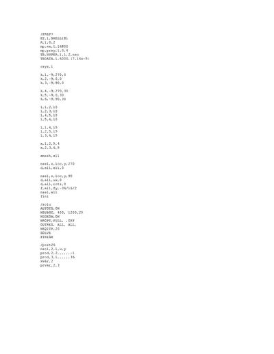
Figure 6. ANSYS input listing for Problem 3.
Figure 7. ANSYS input listing for Problem 3.


![{\displaystyle \mathbf {F} =\left[{\begin{aligned}{\frac {\partial x}{\partial X}}&&{\frac {\partial x}{\partial Y}}&&{\frac {\partial x}{\partial Z}}\\{\frac {\partial y}{\partial X}}&&{\frac {\partial y}{\partial Y}}&&{\frac {\partial y}{\partial Z}}\\{\frac {\partial z}{\partial X}}&&{\frac {\partial z}{\partial Y}}&&{\frac {\partial z}{\partial Z}}\end{aligned}}\right]~.}](https://wikimedia.org/api/rest_v1/media/math/render/svg/6be3e3ebbc85206c18d4bef044b2e1e26769c18f)


![{\displaystyle {\begin{aligned}x({\boldsymbol {\xi }},t)&=x_{1}(t)~\left[1-{\cfrac {X({\boldsymbol {\xi }})}{2}}-Y({\boldsymbol {\xi }})\right]+x_{2}(t)~{\cfrac {X({\boldsymbol {\xi }})}{2}}+x_{3}(t)~Y({\boldsymbol {\xi }})\\y({\boldsymbol {\xi }},t)&=y_{1}(t)~\left[1-{\cfrac {X({\boldsymbol {\xi }})}{2}}-Y({\boldsymbol {\xi }})\right]+y_{2}(t)~{\cfrac {X({\boldsymbol {\xi }})}{2}}+y_{3}(t)~Y({\boldsymbol {\xi }})\\z({\boldsymbol {\xi }},t)&=Z({\boldsymbol {\xi }})\end{aligned}}}](https://wikimedia.org/api/rest_v1/media/math/render/svg/5985cc7e88e6bae9cbf6fe652049f263f0712607)


![{\displaystyle {\begin{aligned}x({\boldsymbol {\xi }},t)&=\left[2(1+at)\cos {\cfrac {\pi t}{2}}\right]~{\cfrac {X({\boldsymbol {\xi }})}{2}}-\left[(1+bt)\sin {\cfrac {\pi t}{2}}\right]~Y({\boldsymbol {\xi }})\\y({\boldsymbol {\xi }},t)&=\left[2(1+at)\sin {\cfrac {\pi t}{2}}\right]~{\cfrac {X({\boldsymbol {\xi }})}{2}}+\left[(1+bt)\cos {\cfrac {\pi t}{2}}\right]~Y({\boldsymbol {\xi }})\\z({\boldsymbol {\xi }},t)&=Z({\boldsymbol {\xi }})~.\end{aligned}}}](https://wikimedia.org/api/rest_v1/media/math/render/svg/4b0bcdb9b83a103047ab91887aef086b49b25dc7)


![{\displaystyle {\mathbf {F} (t)=\left[{\begin{aligned}(1+at)~\cos {\cfrac {\pi t}{2}}&&-(1+bt)~\sin {\cfrac {\pi t}{2}}&&0\\(1+at)~\sin {\cfrac {\pi t}{2}}&&(1+bt)~\cos {\cfrac {\pi t}{2}}&&0\\0&&0&&1\end{aligned}}\right]~.}}](https://wikimedia.org/api/rest_v1/media/math/render/svg/36e7618d3057cb887742b4cb80912467168888bd)
![{\displaystyle J(t)=\det \mathbf {F} (t)=\left[(1+at)~\cos {\cfrac {\pi t}{2}}\right]\left[(1+bt)~\cos {\cfrac {\pi t}{2}}\right]+\left[(1+bt)~\sin {\cfrac {\pi t}{2}}\right]\left[(1+at)~\sin {\cfrac {\pi t}{2}}\right]~.}](https://wikimedia.org/api/rest_v1/media/math/render/svg/f5db7e773b9c5ced2a03c80cbd186926b62a2fa8)


![{\displaystyle \mathbf {F} (t)=\left[{\begin{aligned}(1+at)~\cos {\cfrac {\pi t}{2}}&&-(1+bt)~\sin {\cfrac {\pi t}{2}}&&0\\(1+at)~\sin {\cfrac {\pi t}{2}}&&(1+bt)~\cos {\cfrac {\pi t}{2}}&&0\\0&&0&&1\end{aligned}}\right]~.}](https://wikimedia.org/api/rest_v1/media/math/render/svg/edeb105e6d0b19750859128fa26889e3c3e45e95)


![{\displaystyle {\begin{aligned}v_{x}(\mathbf {X} ,t)={\frac {\partial x}{\partial t}}&=X~\left[a~\cos {\cfrac {\pi t}{2}}-(1+at)~{\cfrac {\pi }{2}}~\sin {\cfrac {\pi t}{2}}\right]-Y~\left[b~\sin {\cfrac {\pi t}{2}}+(1+bt)~{\cfrac {\pi }{2}}~\cos {\cfrac {\pi t}{2}}\right]\\v_{y}(\mathbf {X} ,t)={\frac {\partial y}{\partial t}}&=X~\left[a~\sin {\cfrac {\pi t}{2}}+(1+at)~{\cfrac {\pi }{2}}~\cos {\cfrac {\pi t}{2}}\right]+Y~\left[b~\cos {\cfrac {\pi t}{2}}-(1+bt)~{\cfrac {\pi }{2}}~\sin {\cfrac {\pi t}{2}}\right]\\v_{z}\mathbf {X} ,t)={\frac {\partial z}{\partial t}}&=0\end{aligned}}}](https://wikimedia.org/api/rest_v1/media/math/render/svg/238d759b95eb784b148ebd0efc75fa0a08e6dbbb)
![{\displaystyle \mathbf {l} ={\boldsymbol {\nabla }}\mathbf {v} =\left[{\begin{aligned}{\frac {\partial v_{x}}{\partial x}}&&{\frac {\partial v_{x}}{\partial y}}&&{\frac {\partial v_{x}}{\partial z}}\\{\frac {\partial v_{y}}{\partial x}}&&{\frac {\partial v_{y}}{\partial y}}&&{\frac {\partial v_{y}}{\partial z}}\\{\frac {\partial v_{z}}{\partial x}}&&{\frac {\partial v_{z}}{\partial y}}&&{\frac {\partial v_{z}}{\partial z}}\end{aligned}}\right]}](https://wikimedia.org/api/rest_v1/media/math/render/svg/b3167e1242fe81315512d453bd16cff294272428)


![{\displaystyle {\dot {\mathbf {F} }}=\left[{\begin{aligned}a~\cos {\cfrac {\pi t}{2}}-(1+at)~{\cfrac {\pi }{2}}~\sin {\cfrac {\pi t}{2}}&&-b~\sin {\cfrac {\pi t}{2}}-(1+bt)~{\cfrac {\pi }{2}}~\cos {\cfrac {\pi t}{2}}&&0\\a~\sin {\cfrac {\pi t}{2}}+(1+at)~{\cfrac {\pi }{2}}~\cos {\cfrac {\pi t}{2}}&&b~\cos {\cfrac {\pi t}{2}}-(1+bt)~{\cfrac {\pi }{2}}~\sin {\cfrac {\pi t}{2}}&&0\\0&&0&&0\end{aligned}}\right]~.}](https://wikimedia.org/api/rest_v1/media/math/render/svg/348622337da1793eeecfbe78a445fa56f5c88999)
![{\displaystyle \mathbf {F} ^{-1}={\cfrac {1}{(1+at)(1+bt)}}\left[{\begin{aligned}(1+bt)~\cos {\cfrac {\pi t}{2}}&&(1+bt)~\sin {\cfrac {\pi t}{2}}&&0\\-(1+at)~\sin {\cfrac {\pi t}{2}}&&(1+at)~\cos {\cfrac {\pi t}{2}}&&0\\0&&0&&(1+at)(1+bt)\end{aligned}}\right]~.}](https://wikimedia.org/api/rest_v1/media/math/render/svg/d228a0fe4db3e700e1dae57d51f437b87c3c9b30)

![{\displaystyle {\dot {\mathbf {F} }}=\left[{\begin{aligned}a~c-A~s~{\cfrac {\pi }{2}}&&-b~s-B~c~{\cfrac {\pi }{2}}&&0\\a~s+A~c~{\cfrac {\pi }{2}}&&b~c-B~s~{\cfrac {\pi }{2}}&&0\\0&&0&&0\end{aligned}}\right]=\left[{\begin{aligned}a~c&&-b~s&&0\\a~s&&b~c&&0\\0&&0&&0\end{aligned}}\right]+{\cfrac {\pi }{2}}\left[{\begin{aligned}-A~s&&-B~c&&0\\A~c&&-B~s&&0\\0&&0&&0\end{aligned}}\right]}](https://wikimedia.org/api/rest_v1/media/math/render/svg/c73ff5c0630d6b611f8e5e29f48cf4b5ee756bcd)
![{\displaystyle \mathbf {F} ^{-1}={\cfrac {1}{A~B}}\left[{\begin{aligned}B~c&&B~s&&0\\-A~s&&A~c&&0\\0&&0&&A~B\end{aligned}}\right]~.}](https://wikimedia.org/api/rest_v1/media/math/render/svg/c3c05f4ea41874502cf54d84f32d99763790ade1)
![{\displaystyle \mathbf {l} ={\cfrac {1}{A~B}}\left[{\begin{aligned}B~a~c^{2}+A~b~s^{2}&&B~a~c~s-A~b~c~s&&0\\B~a~c~s-A~b~c~s&&B~a~s^{2}+A~b~c^{2}&&0\\0&&0&&0\end{aligned}}\right]+{\cfrac {\pi }{2}}\left[{\begin{aligned}0&&-1&&0\\1&&0&&0\\0&&0&&0\end{aligned}}\right]}](https://wikimedia.org/api/rest_v1/media/math/render/svg/19c43af426eb88b0b6e0906720ee8a6de9b4650b)
![{\displaystyle {\mathbf {l} =\left[{\begin{aligned}{\cfrac {a}{1+at}}~\cos ^{2}{\cfrac {\pi t}{2}}+{\cfrac {b}{1+bt}}~\sin ^{2}{\cfrac {\pi t}{2}}&&\left[{\cfrac {a}{1+at}}-{\cfrac {b}{1+bt}}\right]\cos {\cfrac {\pi t}{2}}~\sin {\cfrac {\pi t}{2}}-{\frac {\pi }{2}}&&0\\\left[{\cfrac {a}{1+at}}-{\cfrac {b}{1+bt}}\right]\cos {\cfrac {\pi t}{2}}~\sin {\cfrac {\pi t}{2}}+{\cfrac {\pi }{2}}&&{\cfrac {a}{1+at}}~\sin ^{2}{\cfrac {\pi t}{2}}+{\cfrac {b}{1+bt}}~\cos ^{2}{\cfrac {\pi t}{2}}&&0\\0&&0&&0\end{aligned}}\right]}}](https://wikimedia.org/api/rest_v1/media/math/render/svg/e4c6f741461cf30e6ce996de783057c20ecd2c21)
![{\displaystyle {\mathbf {d} =\left[{\begin{aligned}{\cfrac {a}{1+at}}~\cos ^{2}{\cfrac {\pi t}{2}}+{\cfrac {b}{1+bt}}~\sin ^{2}{\cfrac {\pi t}{2}}&&\left[{\cfrac {a}{1+at}}-{\cfrac {b}{1+bt}}\right]\cos {\cfrac {\pi t}{2}}~\sin {\cfrac {\pi t}{2}}&&0\\\left[{\cfrac {a}{1+at}}-{\cfrac {b}{1+bt}}\right]\cos {\cfrac {\pi t}{2}}~\sin {\cfrac {\pi t}{2}}&&{\cfrac {a}{1+at}}~\sin ^{2}{\cfrac {\pi t}{2}}+{\cfrac {b}{1+bt}}~\cos ^{2}{\cfrac {\pi t}{2}}&&0\\0&&0&&0\end{aligned}}\right]}}](https://wikimedia.org/api/rest_v1/media/math/render/svg/03e836b0c41b887901788cf8fb2f75621e84756b)
![{\displaystyle {\mathbf {w} ={\cfrac {\pi }{2}}\left[{\begin{aligned}0&&-1&&0\\1&&0&&0\\0&&0&&0\end{aligned}}\right]}}](https://wikimedia.org/api/rest_v1/media/math/render/svg/7012d58248927c237b9737c5ed8dc94acdd8cebe)


![{\displaystyle \mathbf {F} (t)=\left[{\begin{aligned}(1+t)~\cos {\cfrac {\pi t}{2}}&&-(1+2t)~\sin {\cfrac {\pi t}{2}}&&0\\(1+t)~\sin {\cfrac {\pi t}{2}}&&(1+2t)~\cos {\cfrac {\pi t}{2}}&&0\\0&&0&&1\end{aligned}}\right]~.}](https://wikimedia.org/api/rest_v1/media/math/render/svg/c99230d2f73820d2b1b5299fa407015a059b49ec)


=0~.}](https://wikimedia.org/api/rest_v1/media/math/render/svg/fa3dbd3a94c60dca83eb60914d754ced05696f27)


![{\displaystyle \mathbf {N} _{1}=[1~~0~~0]^{T}~;~~\mathbf {N} _{2}=[0~~1~~0]^{T}~;~~\mathbf {N} _{3}=[0~~0~~1]^{T}~.}](https://wikimedia.org/api/rest_v1/media/math/render/svg/79fbfad61b6e73a9f6a78bd1d9004cb6d3f4d295)


![{\displaystyle {\mathbf {R} =\left[{\begin{aligned}\cos {\cfrac {\pi t}{2}}&&-\sin {\cfrac {\pi t}{2}}&&0\\\sin {\cfrac {\pi t}{2}}&&\cos {\cfrac {\pi t}{2}}&&0\\0&&0&&1\end{aligned}}\right]~.}}](https://wikimedia.org/api/rest_v1/media/math/render/svg/ba6a6f24e305f7c7fccebbff2e195f8021f68bd2)


![{\displaystyle \mathbf {d} =\left[{\begin{aligned}{\cfrac {a}{1+at}}~\cos ^{2}{\cfrac {\pi t}{2}}+{\cfrac {b}{1+bt}}~\sin ^{2}{\cfrac {\pi t}{2}}&&\left[{\cfrac {a}{1+at}}-{\cfrac {b}{1+bt}}\right]\cos {\cfrac {\pi t}{2}}~\sin {\cfrac {\pi t}{2}}&&0\\\left[{\cfrac {a}{1+at}}-{\cfrac {b}{1+bt}}\right]\cos {\cfrac {\pi t}{2}}~\sin {\cfrac {\pi t}{2}}&&{\cfrac {a}{1+at}}~a~\sin ^{2}{\cfrac {\pi t}{2}}+{\cfrac {b}{1+bt}}~\cos ^{2}{\cfrac {\pi t}{2}}&&0\\0&&0&&0\end{aligned}}\right]}](https://wikimedia.org/api/rest_v1/media/math/render/svg/ac9f7c107095e6fa1eaa728a5463d61e0239b7ba)
![{\displaystyle \mathbf {d} =\left[{\begin{aligned}{\cfrac {1}{2}}~\cos ^{2}{\cfrac {\pi }{2}}+{\cfrac {2}{3}}~\sin ^{2}{\cfrac {\pi }{2}}&&\left[{\cfrac {1}{2}}-{\cfrac {2}{3}}\right]\cos {\cfrac {\pi }{2}}~\sin {\cfrac {\pi }{2}}&&0\\\left[{\cfrac {1}{2}}-{\cfrac {2}{3}}\right]\cos {\cfrac {\pi }{2}}~\sin {\cfrac {\pi }{2}}&&{\cfrac {1}{2}}~\sin ^{2}{\cfrac {\pi }{2}}+{\cfrac {2}{3}}~\cos ^{2}{\cfrac {\pi }{2}}&&0\\0&&0&&0\end{aligned}}\right]={\begin{bmatrix}{\cfrac {2}{3}}&0&0\\0&{\cfrac {1}{2}}&0\\0&0&0\end{bmatrix}}}](https://wikimedia.org/api/rest_v1/media/math/render/svg/41b16713cb668dd300da589fedfb089ff9d2a688)


![{\displaystyle \mathbf {w} ={\cfrac {\pi }{2}}\left[{\begin{aligned}0&&-1&&0\\1&&0&&0\\0&&0&&0\end{aligned}}\right]}](https://wikimedia.org/api/rest_v1/media/math/render/svg/81098e86e83f3e1a4a67eb20c9c6a79b7095b42a)


![{\displaystyle \mathbf {l} =\left[{\begin{aligned}{\cfrac {a}{1+at}}~\cos ^{2}{\cfrac {\pi t}{2}}+{\cfrac {b}{1+bt}}~\sin ^{2}{\cfrac {\pi t}{2}}&&\left[{\cfrac {a}{1+at}}-{\cfrac {b}{1+bt}}\right]\cos {\cfrac {\pi t}{2}}~\sin {\cfrac {\pi t}{2}}-{\frac {\pi }{2}}&&0\\\left[{\cfrac {a}{1+at}}-{\cfrac {b}{1+bt}}\right]\cos {\cfrac {\pi t}{2}}~\sin {\cfrac {\pi t}{2}}+{\cfrac {\pi }{2}}&&{\cfrac {a}{1+at}}~\sin ^{2}{\cfrac {\pi t}{2}}+{\cfrac {b}{1+bt}}~\cos ^{2}{\cfrac {\pi t}{2}}&&0\\0&&0&&0\end{aligned}}\right]}](https://wikimedia.org/api/rest_v1/media/math/render/svg/b6f8622caeabaeedac9cbd342137c57ee393de7b)
![{\displaystyle \mathbf {l} =\left[{\begin{aligned}{\cfrac {1}{2}}~\cos ^{2}{\cfrac {\pi }{2}}+{\cfrac {2}{3}}~\sin ^{2}{\cfrac {\pi }{2}}&&\left[{\cfrac {1}{2}}-{\cfrac {2}{3}}\right]\cos {\cfrac {\pi }{2}}~\sin {\cfrac {\pi }{2}}-{\frac {\pi }{2}}&&0\\\left[{\cfrac {1}{2}}-{\cfrac {2}{3}}\right]\cos {\cfrac {\pi }{2}}~\sin {\cfrac {\pi }{2}}+{\cfrac {\pi }{2}}&&{\cfrac {1}{2}}~\sin ^{2}{\cfrac {\pi }{2}}+{\cfrac {2}{3}}~\cos ^{2}{\cfrac {\pi }{2}}&&0\\0&&0&&0\end{aligned}}\right]={\begin{bmatrix}{\cfrac {2}{3}}&-{\cfrac {\pi }{2}}&0\\{\cfrac {\pi }{2}}&{\cfrac {1}{2}}&0\\0&0&0\end{bmatrix}}~.}](https://wikimedia.org/api/rest_v1/media/math/render/svg/2b69c860fb868fccd404389f5a2c7d4fabf3300c)