Monetary Circuit Model/Skeleton Model

This lesson explains how to set up a skeleton of the monetary circuit model in Sage. This model looks at an economy with three sectors - banks, firms, and workers - with no monetary transactions taking place in between them. While the model itself is useless, the code given here will form the basis of future models.

The basic mathematical tool used by the monetary circuit model are systems of Ordinary Differential Equations (ODEs). The ODE system describes the flows between sectors of the economy. Taken together with some initial values, Sage can solve the system to describe how stocks (accounts) change over time. To do this, we must first tell Sage the names of the variables and functions we wish to use:

t = var('t')

# The first argument to function() is the symbol displayed when rendered.
# e.g, 'B_v' is displayed as B subscript v. The second argument is the
# function parameter(s)
bv = function('B_v', t)
bt = function('B_t', t)
fl = function('F_l', t)
fd = function('F_d', t)
wd = function('W_d', t)

ibc = 100

This declares our dependent variable, t, for time. Five stocks/accounts are also declared as functions of time: the bank vault, bank transactions account, firm debt (loans), firm deposits, and worker deposits. The constant ibc is the initial bank capital, the amount of money in its vault at the beginning of the first period. It is not used until later, but kept here so all declarations are in one place.

Next, we create a skeleton ODE system:

des = [
	diff(bv, t) == 0,
	diff(bt, t) == 0,
	diff(fl, t) == 0,
	diff(fd, t) == 0,
	diff(wd, t) == 0
	]

This creates a list of differential equations named des, one equation for each of the five stocks. Notice that we use the double-equals sign to specify that this is an equation rather than an assignment.

The system of differential equations specifies our flows. The left hand side of each equation is the first derivative of each stock with respect to time - how quickly the stock changes. The right hand side specifies the flow of money into and out of that stock. For our skeleton system, we do not have any transactions taking place, so the right hand side is 0.

Next, we solve the system:

sol = desolve_system(des,
	[bv, bt, fl, fd, wd],
	[0, ibc, 0 , 0 , 0 , 0],
	t)

The desolve_system() function is somewhat complicated. The first argument is the system of differential equations we want to solve. The second argument is a list of the dependant variables, in this case our five accounts. The third argument is a list of initial conditions. The first element of the list is the initial value of the independant variable (t), followed by the value of the five dependant variables at the initial time t = 0.

We initialize all the stocks to 0 except for the bank vault, which we initialize to the initial bank capital (ibc) declared above.

Finally, we add some code to plot the system:

# This function takes an expression (the right-hand side of the solution),
# a label, and a hue and plots the expression from 0 to 10. Its first derivative
# is also plotted as a separate line, dotted and faded.
def buildplot(expression, label, h):
	global t
	
	# Plot the expression. Remove legend_label and restart the interpreter if
	# you get errors about LaTeX not being installed.
	p = plot(expression, t, (0, 10), rgbcolor=hue(h), legend_label=label)

	# Plot the derivative of the expression at 30% saturation with a dashed line
	p += plot(diff(expression, t), t, (0, 10),
			rgbcolor=hue(h, 0.3), linestyle='--')
	
	return p

# Helper function to generate a unique hue for each curve
def colourwheel(colours):
	for c in xrange(0, colours):
		yield float(c) / colours

# The labels to use. This list should match the list of
# dependant variables used when solving.
labels = ["Bank Vault", "Bank Transactions", "Firm Debt", 
		"Firm Deposits", "Worker Deposits"]

# Create a list of plots, one for each function
plots = [buildplot(s.rhs(), label, c)
		for s, label, c in zip(sol, labels, colourwheel(len(sol)))]

# Combine the individual plots into a single graph
p = plots[0]
for pl in plots[1:]:
	p += pl

# Uncomment to save as graph.svg
# p.save('graph.svg')

# Display the graph
p.show()

You do not have to understand this last bit of code to understand the model. To show the results, save all of the code in a file such as skeleton.py and run the following in the Sage interpreter:

attach skeleton.py

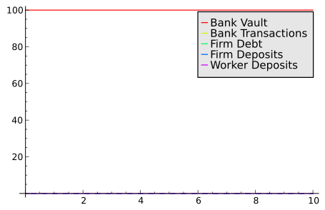
Note: once attached, Sage will automatically reload the file if it is changed. If you make a change, simply press 'enter' in the interpreter to re-run the model. The resulting graph should look something like this:

So far, this is a pretty useless model, since it describes an economy with no monetary transactions. In the next lesson, we will extend the skeleton to create a simple model where banks create money by lending to firms.