File:Late glacial temperature curve1.jpg
Original file (1,600 × 766 pixels, file size: 344 KB, MIME type: image/jpeg)
| This is a file from the Wikimedia Commons. The description on its description page there is shown below.
Commons is a freely licensed media file repository. You can help. |
Summary
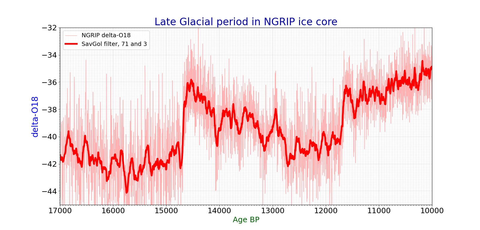
| Description | Temperature curve of late glacial period, from NGRIP greenland ice core oxygen isotope ratio. Numbers thousands of years ago, time goes from right to left, up is warmer, down is colder. The periot spans from Lascaux interstadial to Heinrich event H1, and to Meiendorf/Bölling warm stage, and Allegöd warm stage, to Younger dryas and early holocene. |
| Date | 3 December 2007 (upload date) |
| Source | Own work |
| Author | Merikanto |
Additional info
Source of data is
http://www.iceandclimate.nbi.ku.dk/data/ http://www.iceandclimate.nbi.ku.dk/data/NGRIP_d18O_and_dust_5cm.xls
δ18O values and dust concentrations
The dataset provides NGRIP δ18O
values, dust concentrations, and GICC05 ages in 5cm depth resolution for the
period 0-60 ka (δ18O) and 10-60 ka (dust).
The dataset accompany the following papers:
NGRIP members, Nature, 431, 147-151, 2004. DOI: 10.1038/nature02805
Gkinis et al., Earth Planet. Sci. Lett., 405, 132-141, 2014.  DOI:
10.1016/j.epsl.2014.08.022
Ruth et al., J. Geophys. Res., 108, 4098, 2003. DOI: 4010.1029/2002JD002376
Python code
- drawing climate diagram in python 3
- version 2.11
- 11.9.2020
-
import matplotlib.pyplot as plt
import numpy as np
import pandas as pd
from scipy import interpolate
from matplotlib.ticker import (MultipleLocator, AutoMinorLocator)
import scipy.signal
def running_mean(x, N):
   cumsum = np.cumsum(np.insert(x, 0, 0))
   return (cumsum[N:] - cumsum[:-N]) / float(N)
datafilename="ngrip1.csv"
captioni="Late Glacial period in NGRIP ice core"
savename="ngrip_dryas.svg"
figsizex=16
figsizey=8
- x = []
- y = []
- y2= []
dfin0=pd.read_csv(datafilename, sep=";")
lst1=['gicc05_age','delta_O18']
dfin1 = dfin0[dfin0.columns.intersection(lst1)]
x0=dfin1['gicc05_age']
y0=dfin1['delta_O18']
- y20=dfin1['GISP_dO18']
- y30=dfin1['GISP2_dO18']
x=np.array(x0)
y=np.array(y0)
- y2=np.array(y20)
- y3=np.array(y30)
- list1=[]
- list1.append(y)
- list1.append(y2)
- list1.append(y3)
- data1=np.array(list1)
- print (np.shape(data1))
- data_avg1=np.average(data1, axis=0)
- print(x)
- print(y)
- quit(0)
size0=14
size1=16
size2=18
size3=24
- y_savgol = scipy.signal.savgol_filter(y,31, 3)
y_savgol = scipy.signal.savgol_filter(y,71, 3)
- y_running = running_mean(y, 31)
x_sm = np.array(x)
y_sm = np.array(y)
x_smooth = np.linspace(x_sm.min(), x_sm.max(), 20000)
funk1 = interpolate.interp1d(x_sm, y_sm, kind="cubic")
y_smooth = funk1(x_smooth)


fig, ax1 = plt.subplots()
- ax1.axis((11600,14000,0,ymax1))
ax1.set_xlim(10000,17000)
ax1.set_ylim(-32.0, -45.0)
- ax1.set_ylim(-35.0, -42.0)
plt.gca().invert_xaxis()
plt.gca().invert_yaxis()
ax1.set_ylabel('delta-O18', color='#0000ff', fontsize=size2+2)


ax1.plot(x,y, color="#ffb0b0", linewidth=1,label="NGRIP delta-O18")
- ax1.plot(x_smooth,y_smooth, color="#0000ff", linewidth=3,label="NGRIP delta-O18")
ax1.plot(x,y_savgol, color="#FF0000", linewidth=4, label="SavGol filter, 71 and 3")
- ax1.plot(x,y_running, color="#FF0000", linewidth=3)
- ax1.plot(x,data_avg1, color="#ff0000", linewidth=2, linestyle=":", label="Average of NGRIP, GISP, GISP2 delta-O18")
ax1.tick_params(axis='both', which='major', labelsize=size2)
ax1.xaxis.set_minor_locator(MultipleLocator(500))
ax1.xaxis.set_minor_locator(MultipleLocator(50))
ax1.yaxis.set_minor_locator(MultipleLocator(1.0))
ax1.yaxis.set_minor_locator(MultipleLocator(0.1))
ax1.grid(which='major', linestyle='-', linewidth='0.1', color='black')
ax1.grid(which='minor', linestyle=':', linewidth='0.1', color='black')


ax1.set_xlabel('Age BP', color="darkgreen", fontsize=size2)


ax1.set_title(captioni, fontsize=size3, color="#0000af")
plt.legend(fontsize=size0)
fig = plt.gcf()
fig.set_size_inches(figsizex, figsizey, forward=True)


plt.savefig(savename, format="svg", dpi = 100)
plt.show()
Licensing
| I, the copyright holder of this work, release this work into the public domain. This applies worldwide. In some countries this may not be legally possible; if so: I grant anyone the right to use this work for any purpose, without any conditions, unless such conditions are required by law. |
File history
Click on a date/time to view the file as it appeared at that time.
| Date/Time | Thumbnail | Dimensions | User | Comment | |
|---|---|---|---|---|---|
| current | 17:25, 12 September 2020 | | 1,600 × 766 (344 KB) | Merikanto | New data and layoyut |
| 21:12, 3 December 2007 |  | 910 × 579 (135 KB) | Merikanto~commonswiki | {{Information |Description=Temperature curve of late glacial period, from NGRIP greenland ice core oxygen isotope ratio. Numbers thousands of years ago, time goes from right to left, up is warmer, down is colder. The periot spans from Lascaux interstadial |
File usage
The following 5 pages use this file:
Global file usage
The following other wikis use this file:
- Usage on fi.wikipedia.org