University of Florida/Eml4500/f08.FEABBQ/HW1/Matlab

Homework 1: Matlab Section

Entering matrices

Matlab works completely with matrices.

Matrices are created through 3 different methods. 1. By an entered explicit list of elements 2. By generating a built-in statement or function 3. Loaded from an external file

   A = [ 1 2 3; 4 5 6; 7 8 9]
   A =
       1     2     3
       4     5     6
       7     8     9

Matlab also allows for complex numbers. You may use i or j.

    a = [1 2;3 4] + i*[5 6;7 8]
    a =
       1.0000 + 5.0000i   2.0000 + 6.0000i
       3.0000 + 7.0000i   4.0000 + 8.0000i

If i or j are used as variables. A replacement imaginary unit may be created.

    ii = sqrt(-1)
    ii =
       0 + 1.0000i

Many built in functions are available in MATLAB. The function rand may be used to created a matrix with randomly generated entries.

     rand (3)
     ans =
        0.9501    0.4860    0.4565
        0.2311    0.8913    0.0185
        0.6068    0.7621    0.8214

     rand (2,3)
     ans =
        0.4447    0.7919    0.7382
        0.6154    0.9218    0.1763

Function magic will create a martix with a magic square.

    magic (3)
    ans =
       8     1     6
       3     5     7
       4     9     2

Function hilb will create a Hilbert matrix.

    hilb(3)
    ans =
       1.0000    0.5000    0.3333
       0.5000    0.3333    0.2500
       0.3333    0.2500    0.2000

Individual numbers from a matrix may also be accessed by using a similar command example below.

   A(2,3)
    ans =
       6

Matrix operations, array operations

There are multiple matrix operations available. They can be used for scalars and matrices. They are

Code	Description
`+`	additions
`-`	subtraction
`x`	multiplication
`^`	power
`'`	conjugate transpose
`\`	left division
`/`	right division

Operations can be made to operate entry wise by preceding them with a period.

    [1,2,3,4].^2
    ans =
          1     4     9    16

    [1,2,3,4].*[1,2,3,4]
    ans =
          1     4     9    16

Statements, expressions, variables; saving a session

MATLAB statements are usually of the form variable = expression To suppress printing of a statement you must follow the statement with a semicolon (;). MATLAB IS case sensitive. Therefore when creating variables keep in mind the case of the letter. The statement who will list the variables currently created and available.

   who
      Your variables are:
         A    a    ans  ii

To clear a variable simply write clear variable.

   clear ii
   who
      Your variables are:
         A    a    ans

A runaway display can be stopped by pressing CTRL-C.

Lastly to save a session simply press the same button or go to file->save. If a session is not saved it will be lost, thus losing all variables created.

Matrix building functions

Common matrix building functions
Function	Matrix
eye	identity matrix
zeros	matrix of zeros
ones	matrix of ones
diag	create or extract diagonals
triu	upper triangular part of a matrix
tril	lower triangluar part of a matrix
rand	randomly generated matrix
hilb	Hilbert matrix
magic	magic square

Here are few examples

   B = zeros (size(A))
   B =
         0     0     0
         0     0     0
         0     0     0

   diag(A)
   ans =
         1
         5
         9

   diag(diag(A))
   ans =
         1     0     0
         0     5     0
         0     0     9

   B = [A,zeros(3,2); zeros(2,3), eye(2)]
   B =
         1     2     3     0     0
         4     5     6     0     0
         7     8     9     0     0
         0     0     0     1     0
         0     0     0     0     1

For, while, if and relations

These are all commands that will generally be used in M-files.

FOR will set a limit to the number of iterations that will run in a file. For instance

    for x = 1:n
        q = x^2
    end

This code will make q = x^2 as long x is between 1 and n.

WHILE will set an end to a loop by stating the values needed to exit the loop.

     while 2^n < a
         n = n + 1
     end

This code will raise n by one as long as 2^n is less then a.

IF will not run a code unless the starting conditions mach the relation given with if.

     if n<5
         x = 3 + x
         n = n + 1
     end

RELATIONS Here are a list of the relational operators in MATLAB

< less than

> greater than

<= less than or equal

>= greater than or equal

== equal

~= not equal

Relations may be connected by

& and | or

~ not

Scalar functions

built in functions that operate on scalars or individual elements of a matrix. The most commonly used of these functions are as follows:

sin
asin (arcsin)
exp (exponential)
abs
round
cos
acos (arccos)
log (natural log)
sqrt
floor
tan
atan (arctan)
rem (remainder from division)
sign
ceil

EDU>> y=sin(45)

y =

    0.8509

EDU>> asin(45)

ans =

   1.5708 - 4.4997i

EDU>> abs(-17)

ans =

    17

EDU>> round (17.6)

ans =

    18

Vector functions

functions perform actions on vectors in a "column by column" fashion and produce a row vector. The transpose can be used to operate on a row by row basis. Some of those functions are:

max
min
sort
sum
prod
median
mean
std
any
all

EDU>> max(max(A))

ans =

     9

EDU>> max(A)

ans =

     7     8     9

Matrix functions

The following is a list of matrix functions for Matlab. These functions can be accessed using different commands.

eig (eigenvalues and eigenvectors)
chol (cholesky factorization)
svd (singular value decomposition)
inv (inverse)
lu (LU factorization)
qr (QR factorization)
hess (hessenberg form)
schur (schur decomposition)
rref (reduced row echelon form)
expm (matrix exponential)
sqrtm (matrix square root)
poly (characteristic polynomial)
det (determinant)
size (size)
norm (1-norm, 2-norm F-norm)
cond (condition number in the 2-form)
rank (rank)

EDU>> y = eig(A)

y =

   16.1168
   -1.1168
   -0.0000

EDU>> [U,D] = eig (A)

U =

   -0.2320   -0.7858    0.4082
   -0.5253   -0.0868   -0.8165
   -0.8187    0.6123    0.4082

D =

   16.1168         0         0
         0   -1.1168         0
         0         0   -0.0000

Command line editing and recall

Matlab Editing and function keys:

left/right arrows scrolls the cursor left and right

up/down arrows scrolls up and down from line to line

backspace deletes the character left of the cursor

delete deletes the character left of the cursor

home moves the cursor to the beginning of the line

end moves the cursor to the end of the line

EDU>> m=2; n=3; x=0:.01:2*pi; y=sin(m*x); z=cos(n*x); plot(x,y,x,z)

- - There is a graph for this section I just have to figure out how to add it.***
  - I guess you use the 'upload file' in the up-left corner, -andy

Submatrices and colon notation

Matlab allows for the simple creation of vectors with it's "colon notation", whose main operator is the ":", which means "everything." In the following example, a row vector is generated with a starting value of 0.2 and includes "everything" in between 0.2 and its final value, 1.2. The 0.2 in between the colons represents the step-size, meaning that the next value from the starting value is 0.2 over, and the next value after that is 0.2 over, and so on. Other examples of the use of the colon follow.

EDU>> 0.2:0.2:1.2

ans =

    0.2000    0.4000    0.6000    0.8000    1.0000    1.2000

EDU>> x = [0.0:0.1:2.0]';
EDU>> y=sin(x);
EDU>> [x,y]

ans =

         0         0
    0.1000    0.0998
    0.2000    0.1987
    0.3000    0.2955
    0.4000    0.3894
    0.5000    0.4794
    0.6000    0.5646
    0.7000    0.6442
    0.8000    0.7174
    0.9000    0.7833
    1.0000    0.8415
    1.1000    0.8912
    1.2000    0.9320
    1.3000    0.9636
    1.4000    0.9854
    1.5000    0.9975
    1.6000    0.9996
    1.7000    0.9917
    1.8000    0.9738
    1.9000    0.9463
    2.0000    0.9093

The following are more advanced uses of the colon operator.

    A(1:4,3)   first four entries of the third column
    A(:,3)     third column of A
    A(:,[2 4]) columns 2 and 4 of A

M-files: script files, function files

Matlab has a built-in programming language, wherein commands that are usually typed at the prompt can be saved to a file (called an M-file because of its .m filename) and run all at once. There are two types of M-files: script files and function files.

A script is akin to a recipe, where commands are read top-down and executed in that order. Common commands (as well as more advanced commands) can be placed in a script so that they can be eaily executed. Inside of a script file, functions can also be called. Note that the definition of a function must exist in its own M-file, hence the second type of M-file, the function file. An example of function files follow.

M-File (randint.m)
function a = randint(m,n,a,b)
if nargin < 3, a = 0; b =9; end 
a =floor((b-a+1)*rand(m,n)) + a;

function [mean, stdev] = stat(x)
[m,n] = size(x)
if m == 1
    m = n;
end
mean = sum(x)/m
stdev = sqrt(sum(x.^2)/m - mean.^2);

EDU>> [xm, xd] = stat(x)

m =

    21

n =

     1

mean =

     1

xm =

     1

xd =

    0.6055

EDU>> type eig
eig is a built-in function.
EDU>> type vander

function A = vander(v)
%VANDER Vandermonde matrix.
%   A = VANDER(V) returns the Vandermonde matrix whose columns
%   are powers of the vector V, that is A(i,j) = v(i)^(n-j).
%
%   Class support for input V:
%      float: double, single

%   Copyright 1984-2004 The MathWorks, Inc. 
%   $Revision: 5.9.4.1 $  $Date: 2004/07/05 17:01:29 $

n = length(v);
v = v(:);
A = ones(n,class(v));
for j = n-1:-1:1
    A(:,j) = v.*A(:,j+1);
end

EDU>> type rank

function r = rank(A,tol)
%RANK   Matrix rank.
%   RANK(A) provides an estimate of the number of linearly
%   independent rows or columns of a matrix A.
%   RANK(A,tol) is the number of singular values of A
%   that are larger than tol.
%   RANK(A) uses the default tol = max(size(A)) * eps(norm(A)).
%
%   Class support for input A:
%      float: double, single

%   Copyright 1984-2004 The MathWorks, Inc. 
%   $Revision: 5.11.4.3 $  $Date: 2004/08/20 19:50:33 $

s = svd(A);
if nargin==1
   tol = max(size(A)') * eps(max(s));
end
r = sum(s > tol);

Learning to write scripts and functions in M-files is essential to gaining proficiency in Matlab use.

Text strings, error messages, input

Like other programming environments/languages, Matlab has many ways of handling text. To assign a string of text to a variable, enclose the text in single quotes. This method is useful if the text is to be operated on or changed later on.

    s='This is text';

To directly display text, use the disp() function, which is useful for simple messages. The following is a lighthearted example

    disp('FEABBQ is the best group ever')

When programming, it is often desirable to handle errors and use text to display a readable message.

    error('Sorry, the matrix must be symmetric')

The previous example shows the error message if the code was expecting a symmetric matrix and received otherwise. Another common use of text is to take in user input interactively.

    iter=input('Enter the number of iterations:    ')

The previous examples takes in user input and assigns the data to the variable iter. Normal execution of the program then follows.

Managing M-files

The command ed opens the M-file editor while simultaneously closing down the Matlab prompt. While this frees up RAM, it may be inconvenient to have to reopen Matlab and possibly redefine variables and other workspace entities. In order to keep Matlab open whenever running a command that would normally close Matlab, simply precede the command with an exclamation, !. The following code opens the M-file editor; upon exiting the editor, Matlab is opened up in the same state as it was before closing.

    !ed rotate.m

To sum up the introduction to M-file programming, we present common tools to use: debugging, setting directories and working with files.

    help dbtype    Opens the debugging help information
    pwd    Prints the current working directory.
    cd     Changes the directory.
    dir    Prints the contents of a directory.
    ls     Same as dir.

The following is the output of the help dbtype command.

EDU>> help dbtype
 DBTYPE List M-file with line numbers.
    The DBTYPE command is used to list an M-file function with 
    line numbers to aid the user in setting breakpoints.  There are
    two forms to this command.  They are:
 
    DBTYPE MFILE
    DBTYPE MFILE start:end
 
    where MFILE is the name of the M-file function in question and 
    start and end are line numbers.
 
    DBTYPE FILENAME lists the contents of the M-file given a fullpath name
    or a MATLABPATH relative partial pathname (see PARTIALPATH).
 
    See also dbstep, dbstop, dbcont, dbclear, dbstack, dbup, dbdown,
             dbstatus, dbquit, partialpath.

    Reference page in Help browser
       doc dbtype

Comparing efficiency of algorithms: flops, tic, toe

The term flops is used in computer science to designate the number of floating point operations performed (hence the name flops). In Matlab, the command flops can be used to gauge how computationally intensive a section of code (or an entire M-file or script) is numerically. The usage is detailed as follows:

set the number of flops to 0 with the command flops(0). This should happen at the beginning of your code.
At the terminating point (the point after the code whose flops are desired), simply place the command flops.

A special note, with version 7 of Matlab, flop counts are no longer available, though another method of gauging performance of a section of code is to use the tic and toc commands to time the length of execution. The usage is similar to flops:

At the starting point of the code to test, enter the command tic.
At the point where the desired execution time is located, enter the command toc.

An example of this would be

    tic; 123.54*200; toc
    Elapsed time is 0.000024 seconds.

Output format

Any standard computations performed in Matlab are done in double precision. It is possible to control the appearance of the output with the following commands. The following example used is 132.679819*176.23546 and the format option is followed by the output,

    format short
    ans =  2.3383e+004
    format long
    ans = 2.338288893418174e+004

Other output formatting options
Format	Description
`format short e`	scientific notation w/ four decimal places
`format long e`	scientific notation w/ fifteen decimal places
`format rat`	approximation by ratio of small integers
`format hex`	hexadecimal
`format bank`	fixed dollars and cents
`format +`	+,-,blank

Hard Copy

Sometimes it is desirable to obtain a hardcopy of your Matlab work, i.e. a printed version. With the exception of graphics, it is possible to save everything on screen to a file with the following command,

    diary filename

The diary function can be controlled using the commands diary off and diary on, which determine when to stop and restart the recording of on-screen contents, respectively.

Graphics

Matlab is capable of producing a variety of mathematical graphs and figures in 2 and 3 dimensions. The basic commands to use these functions are:

Types of Matlab Graphs
Function	Description
`plot`	2d plot - default with a blue line
`plot3`	3-D plot
`scatter`	2-D scatter plot with no connecting line
`mesh`	3-D wire mesh graph
`surf`	3-D surface graph

Planar 2d Plots

The plot(x,y) function will create a linear graph if x and y are both 1d vectors of the same length. The first variable in the plot function is the horizontal axis, and the second is graphed on the vertical. The easiest way of producing a 1d vector is using colon notation:

Sine wave

>> x = -4:.01:4; y = sin(x); plot(x,y)
>> title('Sin(x)'); xlabel('x'); ylabel('y');

The following is a graph of a sin wave from -4 to 4. Adding shown in the code above is the syntax for adding titles and axis labels using the title() and xlabel()/ylabel() commands respectively.

Streamlined code exists for graphing functions as well. First, an M-file must be created such as the following:

Graphing a function

function y = expnormal(x)
y = exp(-x.^2);

Using this code would now create a 2d graph from -1.5 to 1.5:

>> fplot('expnormal', [-1.5,1.5])

Parametric curve

2d parametric graphs can also be created in Matlab. The following code and Figure 3 demonstrate:

>> t = 0:.001:2*pi; x = cos(3*t); y = sin(2*t); plot(x,y)

Annotating Graphs

Graphs are easily annotated in Matlab as well. Typing in the following commands will label the active figure. The format is like: title('Title Here');

Matlab Graph Annotation Functions
Function	Description
`title`	Title
`xlabel`	X-axis label
`ylabel`	Y-axis label
`gtext`	Text on graph, using mouse for placement
`text`	Text on graph, at specified coordinates

Other visual features are available as well:

Matlab Graph Axis Modifications
Function	Description
`axis[(x_min,x_max,y_min,y_max)]`	Manually set axis limits
`axis(axis)`	Holds axis limits for future graphs
`axis auto`	Auto-scaled limits (Matlab Default)
`v = axis`	Returns `v` showing current scales
`axis square`	Same scale on each axis
`axis equal`	Identical axes
`axis off`	Disables axes
`axis on`	Enables axes

All of these visual modifications should be performed after the plot command.

Multiple Graphs on the Same Figure

Multiple graphs

There are different ways to place multiple graphs onto the same Matlab figure. The first is to overload the plot() function. The following code and Figure 4 show how this can be done:

>> x = 0:.01:2*pi; y1 = sin(x); 
y2 = sin(2*x); y3 = sin(4*x); 
plot(x,y1,x,y2,x,y3)

The hold on command can also be used. When hold is on, every plot graphed will go onto the active figure. Turning hold off will create a new figure for each new graph, which is the Matlab default.

Using Different Colors and Line Types on Graphs

Sometimes the default blue solid line in Matlab graphs can get a little boring. To add a little variety to your graphs, there are several commands that can be incorporated into the plot() function:

Different Styles

>> x=0:.01:2*pi; y1=sin(x);y2=sin(2*x); y3=sin(4*x);
plot(x,y1,'--',x,y2,':',x,y3,'+')

Matlab Graph Options
Linetypes	(-) Solid	(--) Dashed	(:) Dotted	(-.) Dashdot
Marktypes	(.) Point	(+) Plus	(*) Star	(o) Circle	(x) X-mark
Colors	(y) Yellow	(m) Magenta	(c) Cyan	(r) Red	(g) Green	(b) Blue	(w) White	(k) Black

These commands are used inside single quotation marks inside the plot() function. plot(x,y,'r--') would plot a dashed red line and plot(x,y,'g:') would plot a green dotted line.

Other Types of Graphs

There are several other types of graphs which Matlab can produce. Although this guide does not have the details for them, they can all be easily found using the help command.

Polar
Bar
Hist
Quiver
Compass
Feather
Rose
Stairs
Fill
Subplot

Graphics Hardcopy

Oftentimes it is necessary to print a graph from Matlab. This is most easily done with the convenient 'Print' menu option on the Figure. It is normally easier though to use 'Save as' and save the graph as a .jpg or other type of graphics file. For the more adventurous, Matlab has a print command which will print the active graphics item. The -append option can also be used to append a different saved file to the current graphics item for printing. Just use the format print -append filename.

3-D Line Plots

There are few more impressive ways to show off Matlab skills than producing colorful 3-D plots. The plot3() command can easily plot in 3 dimensions, just like plot() plots in 2 dimensions. The following example shows how a 3-D plot (Figure 6) can be parametrically created:

3-D Spiral

>> t=.01:.01:20*pi; x=cos(t); 
y=sin(t); z=t.^3; plot3(x,y,z)

All of the settings applicable to 2-D plots (including axis labels and commands, titles, colors, etc) can be used on a 3-D plot as well.

3-D Mesh and Surface Plots

The mesh() and surf() functions can create 3 dimensional representations of matrices, either with a wire mesh or solid surface. If a single matrix can be inputed into either function, the z value is the matrix value at point (x,y) (row, col). Figures 7 and 8 show the mesh() and surf() functions being used to graph the 'eye' (identity) matrix:

Mesh Plot

Surface Plot

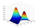
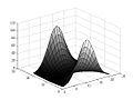
3-D functions can also be graphed using mesh() and surf() in conjunction with the meshgrid() function. Combined with colon notation, meshgrid() creates an x-y rectangle in which a function is graphed. The following code and Figure 9 show how a 3-D function can be defined and graphed:

3-D function graphing

>> [x,y] = meshgrid(-2:.2:2, -2:.2:2);
>> z = exp(x.^2 - y.^2); mesh(z)

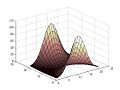
There are several ways to change the appearance of a 3-D graph in Matlab. First of all, the shading command will affect the superimposed mesh lines on a surface graph. Various color profiles can also be experimented with. The following commands can be used like this: colormap(cool)

colormap(hsv)
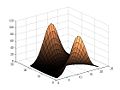
colormap(hot)
colormap(cool)
colormap(jet)
colormap(pink)
colormap(copper)
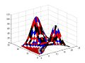colormap(flag)
colormap(gray)
colormap(bone)

Any of the functions to change the appearance should be used after the graph has been made.

Graphs can also be produced parametrically with M-files. Check the guide for further information on this, and Matlab's 'Handle Graphics' which can produce advanced graphs and plots.

Sparse Matrix Computations

Matlab typically handles matrices of which the contents are mostly nonzero. These matrices are considered "dense". A matrix with mostly zero entries is considered "sparse" and is worth defining for the possibility of ignoring the zero values and operating on the nonzero values only. The benefit of this is to reduce the memory footprint of the matrix and the computation time. Suppose a matrix is created by the following command,

    F=floor(10*rand(6))

and that the matrix is filled with mostly zeros by the following command,

    F=triu(tril(F,1),-1)

the output of which looks like

    F =
    9     4     0     0     0     0
    2     0     7     0     0     0
    0     8     1     0     0     0
    0     0     4     3     6     0
    0     0     0     8     2     4
    0     0     0     0     1     4

The nonzero values of the matrix can be easily found with the command, followed by the output,

    S=sparse(F)
    S =
    (1,1)        9
    (2,1)        2
    (1,2)        4
    (3,2)        8
    (2,3)        7
    (3,3)        1
    (4,3)        4
    (4,4)        3
    (5,4)        8
    (4,5)        6
    (5,5)        2
    (6,5)        1
    (5,6)        4
    (6,6)        4

The following commands will return the matrix to it's previous form and check it's storage mode, respectively

    F=full(S)
    issparse(F)

Sparse matrices can also be generated directly as opposed to calling the sparse function on a full ("dense") matrix. A sparse diagonal matrix can be generated with the spdiags command. The output is similar to calling the sparse.

    m=6;n=6;e=ones(n,1);d=-2*e;
    T=spdiags([e,d,e],[-1,0,1],m,n)
    T =
    (1,1)       -2
    (2,1)        1
    (1,2)        1
    (2,2)       -2
    (3,2)        1
    (2,3)        1
    (3,3)       -2
    (4,3)        1
    (3,4)        1
    (4,4)       -2
    (5,4)        1
    (4,5)        1
    (5,5)       -2
    (6,5)        1
    (5,6)        1
    (6,6)       -2

speye,sparse,spones,sprandn are the sparse analogs of eye,zeros,ones and randn, respectively. A more specific approach would be to define the nonzero values of the sparse matrix individually. For example (followed by output)

    i=[1 2 3 4 4 4];j=[1 2 3 1 2 3]; s=[5 6 7 8 9 10];
    full(S),S = sparse(i,j,s,4,3)
    ans =
    5     0     0
    0     6     0
    0     0     7
    8     9    10
    S =
    (1,1)        5
    (4,1)        8
    (2,2)        6
    (4,2)        9
    (3,3)        7
    (4,3)       10

The nonzero entities were stored in the row vector s. Another example of directly defining the nonzero values of a sparse matrix is

    n=6;e=floor(10*rand(n-1,1));E=sparse(2:n,1:n-1,e,n,n)
    E =
    (2,1)        8
    (3,2)        5
    (4,3)        2
    (5,4)        6
    (6,5)        8

The output of Matlab arithmetic and functions will be in one of the two storage modes (either Full(F) or Sparse(S)). The following defines the output results of the manipulation done to either full or sparse matrices

    Sparse: S+S, S*S, S.*S, S.*F, S^n, S.^n, S\S, inv(S), chol(S), lu(S), diag(S)
            max(S), sum(S)
    Full: S+F, S*F, S\F, F\S