File:Snells law wavefronts.gif

Snells_law_wavefronts.gif(225 × 227 pixels, file size: 65 KB, MIME type: image/gif, looped, 10 frames, 0.1 s)

This is a file from the Wikimedia Commons. The description on its description page there is shown below.

Commons is a freely licensed media file repository. You can help.

Titel

Summary

 
This diagram was created with MATLAB.
Description
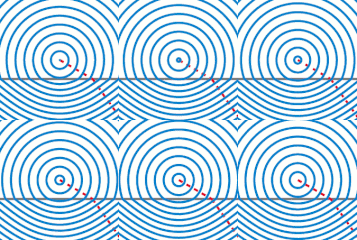
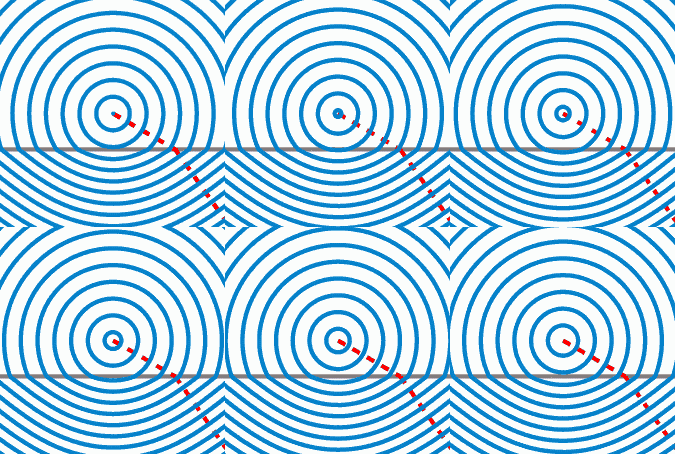
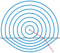
English: Illustration of wavefronts in the context of Snell's law.
Date (UTC)
Source Own work, created with MATLAB. (Source code below.)
Author Oleg Alexandrov
Permission
(Reusing this file)
Public domain I, the copyright holder of this work, release this work into the public domain. This applies worldwide.
In some countries this may not be legally possible; if so:
I grant anyone the right to use this work for any purpose, without any conditions, unless such conditions are required by law.
Other versions

Source code

% Illustration of Snell's law
function main()

   % indexes of refraction
   n1=1.0;
   n2=1.5;

   sign = -1;% is the source up or down?
   O=[0, -1*sign];
   k=500;

   
% KSmrq's colors
   red    = [0.867 0.06 0.14];
   blue   = [0, 129, 205]/256;
   green  = [0, 200,  70]/256;
   yellow = [254, 194,   0]/256;
   white = 0.99*[1, 1, 1];
   black = [0, 0, 0];
   gray = 0.5*white;

   color1=red;
   color2=blue;
   color3=gray;
   lw = 3;
   
   plot_line=0;
   Theta=linspace(0, 2*pi, k);
   V=0*Theta; W=0*Theta;
   S0=7;
   spacing=0.45;
   p=floor(S0/spacing);
   S=linspace(0, S0, p+1);
   spacing=S(2)-S(1);
   
   num_frames = 10;
   for frame_iter=1:num_frames

      figure(1); clf; hold on; axis equal; axis off;

      % plot the interface between diellectrics
      L=1.2*S0;
      plot([-L, L], [0, 0], 'color', color3, 'linewidth', lw);
      
      
      % plot a ray
      plot_line=1;
      s=L;
      theta=pi/3; wfr(s, theta, n1, n2, O, sign, plot_line, color1, lw);

      % plot the wafefronts
      plot_line=0;
      for i=1:p

	 s=S(i)+spacing*(frame_iter-1)/num_frames;

	 for j=1:k
	    theta=Theta(j);
	    [V(j), W(j)]=wfr(s, theta, n1, n2, O, sign, plot_line, color1, lw);
	 end
	 plot(V, W, 'color', color2, 'linewidth', lw);
      end
      

      %  dummy points to enlarge the bounding box
      plot(0, S0+2.5*spacing, '*', 'color', white);
      plot(0, -(S0+2.5*spacing)/n2, '*', 'color', white);

      % to know where to crop later
      Lx=3.2; Ly=Lx; shift = 1;
      plot([-Lx, Lx, Lx, -Lx -Lx], ...
           [-Ly, -Ly, Ly, Ly, -Ly]+shift);

      file = sprintf('Frame%d.eps', 1000+frame_iter);
      disp(file);
      saveas(gcf, file, 'psc2')
   end
end

% Converted to gif with the UNIX command
% convert -density 100 -antialias Frame10* Snell_animation.gif 
% then cropped in Gimp

function [a, b]=wfr(s, theta, n1, n2, O, sign, plot_line, color1, lw);

   X=O+s*[sin(theta), sign*cos(theta)];

  if( sign*X(2) > 0 )
    t=-sign*O(2)/cos(theta);
    X0=O+t*[sin(theta), sign*cos(theta)];
    
    if (plot_line == 1) 
      plot([O(1), X0(1)], [O(2), X0(2)], 'color', color1, 'linewidth', lw, 'linestyle', '--');
    end

    d = norm(O-X0);
    r = (s-d)*(n2/n1)^(sign);

    theta2=asin(n1*sin(theta)/n2);
    XE=X0+r*[sin(theta2), sign*cos(theta2)];
  else
    XE = X;
  end  
  a = XE(1);
  b = XE(2); 

  if (plot_line==1)
    plot([X0(1), XE(1)], [X0(2), XE(2)], 'color', color1, 'linewidth', lw, 'linestyle', '--');
  end  
end

Captions

Wavefronts from a point source of light.In a particuler wavefront u will see that the dist btw source & wavefront above the line is > dist btw source & wavefront below the line beacuse lightspeed is greater in the above and lower in below.

Items portrayed in this file

depicts

File history

Click on a date/time to view the file as it appeared at that time.

Date/TimeThumbnailDimensionsUserComment
current09:59, 5 July 2009Thumbnail for version as of 09:59, 5 July 2009225 × 227 (65 KB)Capmoreduced to 16 colors with no quality loss
06:31, 2 January 2008Thumbnail for version as of 06:31, 2 January 2008225 × 227 (148 KB)Oleg Alexandrov{{Information |Description=Illustration of wavefronts in the context of Snell's law. |Source=self-made with MATLAB |Date=05:36, 1 January 2008 (UTC) |Author= Oleg Alexandrov |Permission= |oth

Global file usage

The following other wikis use this file:

View more global usage of this file.